Data Science

Data analysis is the process of inspecting, cleansing, transforming, and modelling data with a goal of discovering useful information, suggesting conclusions, and supporting decision-making.

Data mining is a particular data analysis technique that focuses on the modelling and knowledge discovery for predictive rather than purely descriptive purposes, while business intelligence covers data analysis that relies heavily on aggregation, focusing on business information.

In statistical applications, data analysis can be divided into:

Descriptive Data Analysis:

Rather than find hidden information in the data, descriptive data analysis looks to summarize the dataset.
They are commonly implemented measures included in the descriptive data analysis:

Central tendency (Mean, Mode, Median)
Variability (Standard deviation, Min/Max)

Exploratory data analysis (EDA):

Generate Summaries and make general statements about the data, and its relationships within the data is the heart of Exploratory Data Analysis.
We generally make assumptions on the entire population but mostly just work with small samples. Why are we allowed to do this??? Two important definitions:

Population: A precise definition of all possible outcomes, measurements or values for which inference will be made about.
Sample: A portion of the population which is representative of the population (at least ideally).

Confirmatory data analysis (CDA):

In statistics, confirmatory analysis (CA) or confirmatory factor analysis (CFA) is a special form of factor analysis, most commonly used in social research.

Central tendency

https://statistics.laerd.com/statistical-guides/measures-central-tendency-mean-mode-median.php

A central tendency (or measure of central tendency) is a single value that attempts to describe a set of data by identifying the central position within that set of data.

The mean (often called the average) is most likely the measure of central tendency that you are most familiar with, but there are others, such as the median and the mode.

The mean, median and mode are all valid measures of central tendency, but under different conditions, some measures of central tendency become more appropriate to use than others. In the following sections, we will look at the mean, mode and median, and learn how to calculate them and under what conditions they are most appropriate to be used.

Mean

Mean (Arithmetic)

The mean (or average) is the most popular and well known measure of central tendency.

The mean is equal to the sum of all the values in the data set divided by the number of values in the data set.

So, if we have $n$ values in a data set and they have values $x_{1},x_{2},...,x_{n},$ the sample mean, usually denoted by ${\bar {x}}$ (pronounced x bar), is:

${\bar {x}}={\frac {(x_{1}+x_{2}+...+x_{n})}{n}}={\frac {\sum x}{n}}$

The mean is essentially a model of your data set. It is the value that is most common. You will notice, however, that the mean is not often one of the actual values that you have observed in your data set. However, one of its important properties is that it minimises error in the prediction of any one value in your data set. That is, it is the value that produces the lowest amount of error from all other values in the data set.

An important property of the mean is that it includes every value in your data set as part of the calculation. In addition, the mean is the only measure of central tendency where the sum of the deviations of each value from the mean is always zero.

When not to use the mean

The mean has one main disadvantage: it is particularly susceptible to the influence of outliers. These are values that are unusual compared to the rest of the data set by being especially small or large in numerical value. For example, consider the wages of staff at a factory below:

Staff	1	2	3	4	5	6	7	8	9	10
Salary	$15k$	$18k$	$16k$	$14k$	$15k$	$15k$	$12k$	$17k$	$90k$	$95k$

The mean salary for these ten staff is $30.7k. However, inspecting the raw data suggests that this mean value might not be the best way to accurately reflect the typical salary of a worker, as most workers have salaries in the $12k to 18k range. The mean is being skewed by the two large salaries. Therefore, in this situation, we would like to have a better measure of central tendency. As we will find out later, taking the median would be a better measure of central tendency in this situation.

Another time when we usually prefer the median over the mean (or mode) is when our data is skewed (i.e., the frequency distribution for our data is skewed). If we consider the normal distribution - as this is the most frequently assessed in statistics - when the data is perfectly normal, the mean, median and mode are identical. Moreover, they all represent the most typical value in the data set. However, as the data becomes skewed the mean loses its ability to provide the best central location for the data because the skewed data is dragging it away from the typical value. However, the median best retains this position and is not as strongly influenced by the skewed values. This is explained in more detail in the skewed distribution section later in this guide.

Mean in R

mean(iris$Sepal.Width)

Median

The median is the middle score for a set of data that has been arranged in order of magnitude. The median is less affected by outliers and skewed data. In order to calculate the median, suppose we have the data below:

65	55	89	56	35	14	56	55	87	45	92

We first need to rearrange that data into order of magnitude (smallest first):

14	35	45	55	55	56	56	65	87	89	92

Our median mark is the middle mark - in this case, 56. It is the middle mark because there are 5 scores before it and 5 scores after it. This works fine when you have an odd number of scores, but what happens when you have an even number of scores? What if you had only 10 scores? Well, you simply have to take the middle two scores and average the result. So, if we look at the example below:

65	55	89	56	35	14	56	55	87	45

We again rearrange that data into order of magnitude (smallest first):

14	35	45	55	55	56	56	65	87	89

Only now we have to take the 5th and 6th score in our data set and average them to get a median of 55.5.

Median in R

median(iris$Sepal.Length)

Mode

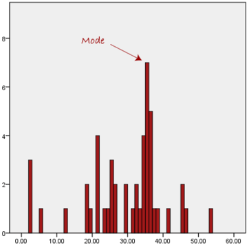
The mode is the most frequent score in our data set. On a histogram it represents the highest bar in a bar chart or histogram. You can, therefore, sometimes consider the mode as being the most popular option. An example of a mode is presented below:

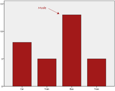
Normally, the mode is used for categorical data where we wish to know which is the most common category, as illustrated below:

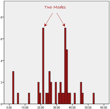
We can see above that the most common form of transport, in this particular data set, is the bus. However, one of the problems with the mode is that it is not unique, so it leaves us with problems when we have two or more values that share the highest frequency, such as below:

We are now stuck as to which mode best describes the central tendency of the data. This is particularly problematic when we have continuous data because we are more likely not to have any one value that is more frequent than the other. For example, consider measuring 30 peoples' weight (to the nearest 0.1 kg). How likely is it that we will find two or more people with exactly the same weight (e.g., 67.4 kg)? The answer, is probably very unlikely - many people might be close, but with such a small sample (30 people) and a large range of possible weights, you are unlikely to find two people with exactly the same weight; that is, to the nearest 0.1 kg. This is why the mode is very rarely used with continuous data.

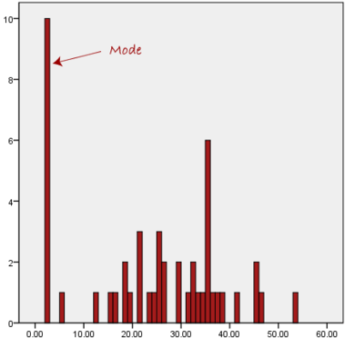
Another problem with the mode is that it will not provide us with a very good measure of central tendency when the most common mark is far away from the rest of the data in the data set, as depicted in the diagram below:

In the above diagram the mode has a value of 2. We can clearly see, however, that the mode is not representative of the data, which is mostly concentrated around the 20 to 30 value range. To use the mode to describe the central tendency of this data set would be misleading.

To get the Mode in R

install.packages("modeest")
library(modeest)

> mfv(iris$Sepal.Width, method = "mfv")

Skewed Distributions and the Mean and Median

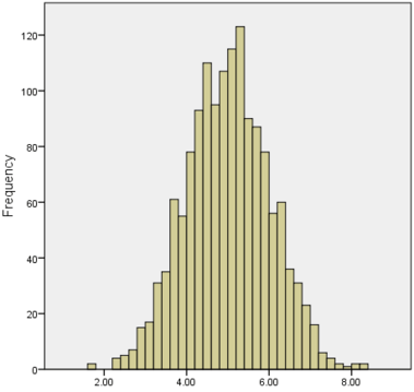
We often test whether our data is normally distributed because this is a common assumption underlying many statistical tests. An example of a normally distributed set of data is presented below:

When you have a normally distributed sample you can legitimately use both the mean or the median as your measure of central tendency. In fact, in any symmetrical distribution the mean, median and mode are equal. However, in this situation, the mean is widely preferred as the best measure of central tendency because it is the measure that includes all the values in the data set for its calculation, and any change in any of the scores will affect the value of the mean. This is not the case with the median or mode.

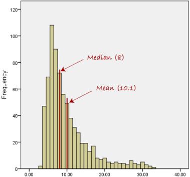
However, when our data is skewed, for example, as with the right-skewed data set below:

we find that the mean is being dragged in the direct of the skew. In these situations, the median is generally considered to be the best representative of the central location of the data. The more skewed the distribution, the greater the difference between the median and mean, and the greater emphasis should be placed on using the median as opposed to the mean. A classic example of the above right-skewed distribution is income (salary), where higher-earners provide a false representation of the typical income if expressed as a mean and not a median.

If dealing with a normal distribution, and tests of normality show that the data is non-normal, it is customary to use the median instead of the mean. However, this is more a rule of thumb than a strict guideline. Sometimes, researchers wish to report the mean of a skewed distribution if the median and mean are not appreciably different (a subjective assessment), and if it allows easier comparisons to previous research to be made.

Summary of when to use the mean, median and mode

Please use the following summary table to know what the best measure of central tendency is with respect to the different types of variable:

Type of Variable	Best measure of central tendency
Nominal	Mode
Ordinal	Median
Interval/Ratio (not skewed)	Mean
Interval/Ratio (skewed)	Median

For answers to frequently asked questions about measures of central tendency, please go to: https://statistics.laerd.com/statistical-guides/measures-central-tendency-mean-mode-median-faqs.php

Measures of Variation

Range

The Range just simply shows the min and max value of a variable.

In R:

> min(iris$Sepal.Width)
> max(iris$Sepal.Width)
> range(iris$Sepal.Width)

Range can be used on Ordinal, Ratio and Interval scales

Quartile

https://statistics.laerd.com/statistical-guides/measures-of-spread-range-quartiles.php

Quartiles tell us about the spread of a data set by breaking the data set into quarters, just like the median breaks it in half.

For example, consider the marks of the 100 students, which have been ordered from the lowest to the highest scores.

The first quartile (Q1): Lies between the 25th and 26th student's marks.
- So, if the 25th and 26th student's marks are 45 and 45, respectively:
  - (Q1) = (45 + 45) ÷ 2 = 45
The second quartile (Q2): Lies between the 50th and 51st student's marks.
- If the 50th and 51th student's marks are 58 and 59, respectively:
  - (Q2) = (58 + 59) ÷ 2 = 58.5
The third quartile (Q3): Lies between the 75th and 76th student's marks.
- If the 75th and 76th student's marks are 71 and 71, respectively:
  - (Q3) = (71 + 71) ÷ 2 = 71

In the above example, we have an even number of scores (100 students, rather than an odd number, such as 99 students). This means that when we calculate the quartiles, we take the sum of the two scores around each quartile and then half them (hence Q1= (45 + 45) ÷ 2 = 45) . However, if we had an odd number of scores (say, 99 students), we would only need to take one score for each quartile (that is, the 25th, 50th and 75th scores). You should recognize that the second quartile is also the median.

Quartiles are a useful measure of spread because they are much less affected by outliers or a skewed data set than the equivalent measures of mean and standard deviation. For this reason, quartiles are often reported along with the median as the best choice of measure of spread and central tendency, respectively, when dealing with skewed and/or data with outliers. A common way of expressing quartiles is as an interquartile range. The interquartile range describes the difference between the third quartile (Q3) and the first quartile (Q1), telling us about the range of the middle half of the scores in the distribution. Hence, for our 100 students:

$Interquartile\ range=Q3-Q1=71-45=26$

However, it should be noted that in journals and other publications you will usually see the interquartile range reported as 45 to 71, rather than the calculated $Interquartile\ range.$

A slight variation on this is the $semi{\text{-}}interquartilerange,$ which is half the $Interquartile\ range.$ Hence, for our 100 students:

$Semi{\text{-}}Interquartile\ range={\frac {Q3-Q1}{2}}={\frac {71-45}{2}}=13$

Quartile in R

quantile(iris$Sepal.Length)

Result 
0%    25%    50%    75%    100% 
4.3   5.1    5.8    6.4    7.9

0% and 100% are equivalent to min max values.

Box Plots

boxplot(iris$Sepal.Length,
       col = "blue", 
       main="iris dataset", 
       ylab = "Sepal Length")

Variance

https://statistics.laerd.com/statistical-guides/measures-of-spread-absolute-deviation-variance.php

Another method for calculating the deviation of a group of scores from the mean, such as the 100 students we used earlier, is to use the variance. Unlike the absolute deviation, which uses the absolute value of the deviation in order to "rid itself" of the negative values, the variance achieves positive values by squaring each of the deviations instead. Adding up these squared deviations gives us the sum of squares, which we can then divide by the total number of scores in our group of data (in other words, 100 because there are 100 students) to find the variance (see below). Therefore, for our 100 students, the variance is 211.89, as shown below:

$variance=\sigma ={\frac {\sum (X-\mu )^{2}}{N}}$

$\mu :{\text{Mean}};\ \ \ X:{\text{Score}};\ \ \ N:{\text{Number of scores}}$

Variance describes the spread of the data.
It is a measure of deviation of a variable from the arithmetic mean.
The technical definition is the average of the squared differences from the mean.
A value of zero means that there is no variability; All the numbers in the data set are the same.
A higher number would indicate a large variety of numbers.

Variance in R

var(iris$Sepal.Length)

Standard Deviation

https://statistics.laerd.com/statistical-guides/measures-of-spread-standard-deviation.php

The standard deviation is a measure of the spread of scores within a set of data. Usually, we are interested in the standard deviation of a population. However, as we are often presented with data from a sample only, we can estimate the population standard deviation from a sample standard deviation. These two standard deviations - sample and population standard deviations - are calculated differently. In statistics, we are usually presented with having to calculate sample standard deviations, and so this is what this article will focus on, although the formula for a population standard deviation will also be shown.

The sample standard deviation formula is:

$s={\sqrt {\frac {\sum (X-{\bar {X}})^{2}}{n-1}}}$

${\bar {X}}:{\text{Sample mean}};\ \ \ n:{\text{Number of scores in the sample}}$

The population standard deviation formula is:

$\sigma ={\sqrt {\frac {\sum (X-\mu )^{2}}{n}}}$

$\mu :{\text{population mean}}$

The Standard Deviation is the square root of the variance.
This measure is the most widely used to express deviation from the mean in a variable.
The higher the value the more widely distributed are the variable data values around the mean.
Assuming the frequency distributions approximately normal, about 68% of all observations are within +/- 1 standard deviation.
Approximately 95% of all observations fall within two standard deviations of the mean (if data is normally distributed).

Standard Deviation in R

sd(iris$Sepal.Length)

Z Score

z-score represents how far from the mean a particular value is based on the number of standard deviations.
z-scores are also known as standardized residuals
Note: mean and standard deviation are sensitive to outliers

> x <-((iris$Sepal.Width) - mean(iris$Sepal.Width))/sd(iris$Sepal.Width)
> x 
> x[77] #choose a single row # or this
> x <-((iris$Sepal.Width[77]) - mean(iris$Sepal.Width))/sd(iris$Sepal.Width)
> x

Shape of Distribution

Skewness

Skewness is a method for quantifying the lack of symmetry in the distribution of a variable.

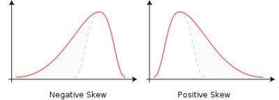
Skewness value of zero indicates that the variable is distributed symmetrically. Positive number indicate asymmetry to the left, negative number indicates asymmetry to the right.

Skewness in R

> install.packages("moments") and library(moments)
> skewness(iris$Sepal.Width)

Histograms in R

> hist(iris$Petal.Width)

Kurtosis

Kurtosis is a measure that gives indication in terms of the peak of the distribution.

Variables with a pronounced peak toward the mean have a high Kurtosis score and variables with a flat peak have a low Kurtosis score.

Kurtosis in R

> kurtosis(iris$Sepal.Length)

Correlations

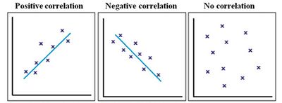
Correlation give us a measure of the relation between two or more variables.

Positive correlation: The points lie close to a straight line, which has a positive gradient. This shows that as one variable increases the other increases.

Negative correlation: The points lie close to a straight line, which has a negative gradient. This shows that as one variable increases the other decreases.

No correlation: There is no pattern to the points. This shows that there is no correlation between the tow variables.

Simple Linear Correlation

Looking for the extent to which two values of the two variables are proportional to each other.

Summarised by a straight line.

This line is called a Regression Line or a Least Squares Line.

It is determined by maintaining the lowest possible sum of squared distances between the data points and the line.

We must use interval scales or ratio scales for this type of analysis.

Simple Linear Correlation in R

Example 1:

> install.packages('ggplot2')
> library(ggplot2)
> data("iris")

> ggplot(iris, aes(x=Sepal.Length, y=Sepal.Width)) + 
         geom_point(color='black') + 
         geom_smooth(method=lm, se=FALSE, fullrange=TRUE)

Example 2:

> library(ggplot2)
> data("iris")
> ggplot(iris, aes(x=Petal.Length, y=Sepal.Length)) + 
         geom_point(color='black') + 
         geom_smooth(method=lm, se=FALSE, fullrange=TRUE)

Data Mining

Data mining is the process of discovering patterns in large data sets involving methods at the intersection of machine learning, statistics, and database systems.[1] Data mining is an interdisciplinary subfield of computer science and statistics with an overall goal to extract information (with intelligent methods) from a data set and transform the information into a comprehensible structure for further use. https://en.wikipedia.org/wiki/Data_mining

Data Mining with R - Luis Torgo

http://www.dcc.fc.up.pt/~ltorgo/DataMiningWithR/

The book is accompanied by a set of freely available R source files that can be obtained at the book's Web site. These files include all the code used in the case studies. They facilitate the "do-it-yourself" approach followed in this book. All data used in the case studies is available at the book's Web site as well. Moreover, we have created an R package called DMwR that contains several functions used in the book as well as the datasets already in R format. You should install and load this package to follow the code in the book (details on how to do this are given in the first chapter).

Installing the DMwR package

One thing that you surely should do is install the package associated with this book, which will give you access to several functions used throughout the book as well as datasets. To install it you proceed as with any other package:

Al tratar de instalarlo en Ubuntu 18.04 se generó un error:

Configuration failed because libcurl was not found. Try installing:
 * deb: libcurl4-openssl-dev (Debian, Ubuntu, etc)

Luego de instalar el paquete mencionado, la instalación completó correctamente:

> install.packages('DMwR')

Chapter 3 - Predicting Stock Market Returns

We will address some of the difficulties of incorporating data mining tools and techniques into a concrete business problem. The spe- cific domain used to illustrate these problems is that of automatic «stock trading systems» (sistemas de comercio de acciones). We will address the task of building a stock trading system based on prediction models obtained with daily stock quotes data. Several models will be tried with the goal of predicting the future returns of the S&P 500 market index (The Standard & Poor's 500, often abbreviated as the S&P 500, or just the S&P, is an American stock market index based on the market capitalizations of 500 large companies having common stock listed on the NYSE or NASDAQ). These predictions will be used together with a trading strategy to reach a decision regarding the market orders to generate.

This chapter addresses several new data mining issues, among which are

How to use R to analyze data stored in a database,
How to handle prediction problems with a time ordering among data observations (also known as time series), and
An example of the difficulties of translating model predictions into decisions and actions in real-world applications.

The Available Data

In our case study we will concentrate on trading the S&P 500 market index. Daily data concerning the quotes of this security are freely available in many places, for example, the Yahoo finance site (http://finance.yahoo.com)

The data we will use is available through different methods:

Reading the data from the book R package (DMwR).
The data (in two alternative formats) is also available at http://www.dcc.fc.up.pt/~ltorgo/DataMiningWithR/datasets3.html
- The first format is a comma separated values (CSV) file that can be read into R in the same way as the data used in Chapter 2.
- The other format is a MySQL database dump file that we can use to create a database with the S&P 500 quotes in MySQL.
Getting the Data directly from the Web (from Yahoo finance site, for example). If you choose to follow this path, you should remember that you will probably be using a larger dataset than the one used in the analysis carried out in this book. Whichever source you choose to use, the daily stock quotes data includes information regarding the following properties:
- Date of the stock exchange session
- Open price at the beginning of the session
- Highest price during the session
- Lowest price
- Closing price of the session
- Volume of transactions
- Adjusted close price4

It is up to you to decide which alternative you will use to get the data. The remainder of the chapter (i.e., the analysis after reading the data) is independent of the storage schema you decide to use.

Reading the data from the DMwR package

La data se encuentra cargada en el paquete DMwR. So, after installing the package DMwR, it is enough to issue:

> library(DMwR)
> data(GSPC)

The first statement is only required if you have not issued it before in your R session. The second instruction will load an object, GSPC, of class xts. You can manipulate it as if it were a matrix or a data frame. Try, for example:

> head(GSPC)
            Open  High   Low Close   Volume Adjusted
1970-01-02 92.06 93.54 91.79 93.00  8050000    93.00
1970-01-05 93.00 94.25 92.53 93.46 11490000    93.46
1970-01-06 93.46 93.81 92.13 92.82 11460000    92.82
1970-01-07 92.82 93.38 91.93 92.63 10010000    92.63
1970-01-08 92.63 93.47 91.99 92.68 10670000    92.68
1970-01-09 92.68 93.25 91.82 92.40  9380000    92.40

Reading the Data from the CSV File

Reading the Data from a MySQL Database

Getting the Data directly from the Web

Handling Time-Dependent Data in R

The data available for this case study depends on time. This means that each observation of our dataset has a time tag attached to it. This type of data is frequently known as time series data. The main distinguishing feature of this kind of data is that order between cases matters, due to their attached time tags. Generally speaking, a time series is a set of ordered observations of a variable $Y$ :

$y_{1},y_{2},...,y_{t-1},y_{t},y_{t+1},...,y_{n}$

where $y_{t}$ is the value of the series variable $Y$ at time $t$ .

The main goal of time series analysis is to obtain a model based on past observations of the variable, $y_{1},y_{2},...,y_{t-1},y_{t}$ , which allows us to make predictions regarding future observations of the variable, $y_{t+1},...,y_{n}$ . In the case of our stocks data, we have what is usually known as a multivariate time series, because we measure several variables at the same time tags, namely the Open, High, Low, Close, Volume, and AdjClose.

R has several packages devoted to the analysis of this type of data, and in effect it has special classes of objects that are used to store type-dependent data. Moreover, R has many functions tuned for this type of objects, like special plotting functions, etc.

Among the most flexible R packages for handling time-dependent data are:

zoo (Zeileis and Grothendieck, 2005) and
xts (Ryan and Ulrich, 2010).

Both offer similar power, although xts provides a set of extra facilities (e.g., in terms of sub-setting using ISO 8601 time strings) to handle this type of data.

In technical terms the class xts extends the class zoo, which means that any xts object is also a zoo object, and thus we can apply any method designed for zoo objects to xts objects. We will base our analysis in this chapter primarily on xts objects.

To install «zoo» and «xts» in R:

install.packages('zoo')
install.packages('xts')

The following examples illustrate how to create objects of class xts:

1 > library(xts)
2 > x1 <- xts(rnorm(100), seq(as.POSIXct("2000-01-01"), len = 100, by = "day"))
3 > x1[1:5]

> x2 <- xts(rnorm(100), seq(as.POSIXct("2000-01-01 13:00"), len = 100, by = "min"))
> x2[1:4]

> x3 <- xts(rnorm(3), as.Date(c("2005-01-01", "2005-01-10", "2005-01-12")))
> x3

The function xts() receives the time series data in the first argument. This can either be a vector, or a matrix if we have a multivariate time series.In the latter case each column of the matrix is interpreted as a variable being sampled at each time tag (i.e., each row). The time tags are provided in the second argument. This needs to be a set of time tags in any of the existing time classes in R. In the examples above we have used two of the most common classes to represent time information in R: the POSIXct/POSIXlt classes and the Date class. There are many functions associated with these objects for manipulating dates information, which you may want to check using the help facilities of R. One such example is the seq() function. We have used this function before to generate sequences of numbers.

As you might observe in the above small examples, the objects may be indexed as if they were “normal” objects without time tags (in this case we see a standard vector sub-setting). Still, we will frequently want to subset these time series objects based on time-related conditions. This can be achieved in several ways with xts objects, as the following small examples try to illustrate:

> x1[as.POSIXct("2000-01-04")]

> x1["2000-01-05"]

> x1["20000105"]

> x1["2000-04"]

x1["2000-02-26/2000-03-03"]

> x1["/20000103"]

Multiple time series can be created in a similar fashion as illustrated below:

> mts.vals <- matrix(round(rnorm(25),2),5,5)
> colnames(mts.vals) <- paste('ts',1:5,sep='')
> mts <- xts(mts.vals,as.POSIXct(c('2003-01-01','2003-01-04', '2003-01-05','2003-01-06','2003-02-16')))
> mts

> mts["2003-01",c("ts2","ts5")]

The functions index() and time() can be used to “extract” the time tags information of any xts object, while the coredata() function obtains the data values of the time series:

> index(mts)

> coredata(mts)

Defining the Prediction Tasks

Generally speaking, our goal is to have good forecasts of the future price of the S&P 500 index so that profitable orders can be placed on time.

What to Predict

The trading strategies we will describe in Section 3.5 assume that we obtain a prediction of the tendency of the market in the next few days. Based on this prediction, we will place orders that will be profitable if the tendency is confirmed in the future.

Let us assume that if the prices vary more than $p\%$ , «we consider this worthwhile in terms of trading (e.g., covering transaction costs)» «consideramos que vale la pena en términos de negociación (por ejemplo, que cubre los costos de transacción)». In this context, we want our prediction models to forecast whether this margin is attainable in the next $k$ days.

Please note that within these $k$ days we can actually observe prices both above and below this percentage. For instance, the closing price at time $t+k$ may represent a variation much lower than $p\%$ , but it could have been preceded by a period of prices representing variations much higher than $p\%$ within the window $t...t+k$

This means that predicting a particular price for a specific future time $t+k$ might not be the best idea. In effect, what we want is to have a prediction of the overall dynamics of the price in the next $k$ days, and this is not captured by a particular price at a specific time.

We will describe a variable, calculated with the quotes data, that can be seen as an indicator (a value) of the tendency in the next $k$ days. The value of this indicator should be related to the confidence we have that the target margin $p$ will be attainable in the next $k$ days.

At this stage it is important to note that when we mention a variation in $p\%$ , we mean above or below the current price. The idea is that positive variations will lead us to buy, while negative variations will trigger sell actions. The indicator we are proposing resumes the tendency as a single value, positive for upward tendencies, and negative for downward price tendencies.

Let the daily average price be approximated by:

${\overline {P}}_{i}={\frac {C_{i}+H_{i}+L_{i}}{3}}$

where $C_{i}$ , $H_{i}$ and $L_{i}$ are the close, high, and low quotes for day $i$ , respectively

Let $V_{i}$ be the set of $k$ percentage variations of today's close to the following $k$ days average prices (often called arithmetic returns):

$V_{i}=\left\{{\frac {{\overline {P}}_{i+j}-C_{i}}{C_{i}}}\right\}_{j=1}^{k}$

Our indicator variable is the total sum of the variations whose absolute value is above our target margin $p\%$

$T_{i}=\sum _{v}\left\{v\in V_{i}:v>p\%\lor v<-p\%\right\}$

The general idea of the variable $T$ is to signal $k$ -days periods that have several days with average daily prices clearly above the target variation. High positive values of $T$ mean that there are several average daily prices that are $p\%$ higher than today's close. Such situations are good indications of potential opportunities to issue a buy order, as we have good expectations that the prices will rise. On the other hand, highly negative values of $T$ suggest sell actions, given the prices will probably decline. Values around zero can be caused by periods with "flat" prices or by conflicting positive and negative variations that cancel each other. The following function implements this simple indicator:

T.ind <- function(quotes, tgt.margin = 0.025, n.days = 10) {
     v <- apply(HLC(quotes), 1, mean)
     r <- matrix(NA, ncol = n.days, nrow = NROW(quotes))
     for (x in 1:n.days) r[, x] <- Next(Delt(v, k = x), x)
     x <- apply(r, 1, function(x) sum(x[x > tgt.margin | x < -tgt.margin]))
     if (is.xts(quotes))
          xts(x, time(quotes))
     else x
}

The target variation margin has been set by default to 2.5%

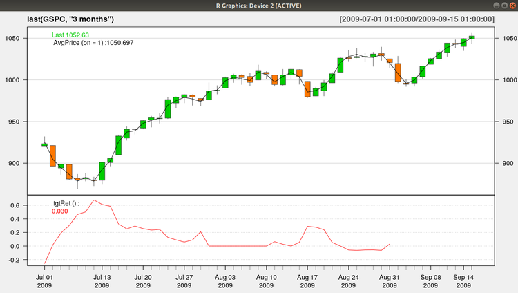
We can get a better idea of the behavior of this indicator in Figure 3.1, which was produced with the following code: https://plot.ly/r/candlestick-charts/

https://stackoverflow.com/questions/44223485/quantmod-r-candlechart-no-colours

Esta creo que es la única librería que hace falta para esta gráfica:

library(quantmod)

> candleChart(last(GSPC, "3 months"), theme = "white", TA = NULL)
> avgPrice <- function(p) apply(HLC(p), 1, mean)
> addAvgPrice <- newTA(FUN = avgPrice, col = 1, legend = "AvgPrice")
> addT.ind <- newTA(FUN = T.ind, col = "red", legend = "tgtRet")
> addAvgPrice(on = 1)
> addT.ind()

S&P500 on the last 3 months and our indicator

Which Predictors?

We have defined an indicator ( $T$ ) that summarizes the behavior of the price time series in the next k days. Our data mining goal will be to predict this behavior. The main assumption behind trying to forecast the future behavior of financial markets is that it is possible to do so by observing the past behavior of the market.

More precisely, we are assuming that if in the past a certain behavior $p$ was followed by another behavior $f$ , and if that causal chain happened frequently, then it is plausible to assume that this will occur again in the future; and thus if we observe $p$ now, we predict that we will observe $f$ next.

We are approximating the future behavior (f ), by our indicator T.

We now have to decide on how we will describe the recent prices pattern (p in the description above). Instead of using again a single indicator to de scribe these recent dynamics, we will use several indicators, trying to capture different properties of the price time series to facilitate the forecasting task.

The simplest type of information we can use to describe the past are the recent observed prices. Informally, that is the type of approach followed in several standard time series modeling approaches. These approaches develop models that describe the relationship between future values of a time series and a window of past q observations of this time series. We will try to enrich our description of the current dynamics of the time series by adding further features to this window of recent prices.

Technical indicators are numeric summaries that reflect some properties of the price time series. Despite their debatable use as tools for deciding when to trade, they can nevertheless provide interesting summaries of the dynamics of a price time series. The amount of technical indicators available can be overwhelming. In R we can find a very good sample of them, thanks to package TTR (Ulrich, 2009).

The indicators usually try to capture some properties of the prices series, such as if they are varying too much, or following some specific trend, etc.

In our approach to this problem, we will not carry out an exhaustive search for the indicators that are most adequate to our task. Still, this is a relevant research question, and not only for this particular application. It is usually known as the feature selection problem, and can informally be defined as the task of finding the most adequate subset of available input variables for a modeling task.

The existing approaches to this problem can usually be cast in two groups: (1) feature filters and (2) feature wrappers.

Feature filters are independent of the modeling tool that will be used after the feature selection phase. They basically try to use some statistical properties of the features (e.g., correlation) to select the final set of features.
The wrapper approaches include the modeling tool in the selection process. They carry out an iterative search process where at each step a candidate set of features is tried with the modeling tool and the respective results are recorded. Based on these results, new tentative sets are generated using some search operators, and the process is repeated until some convergence criteria are met that will define the final set.

We will use a simple approach to select the features to include in our model. The idea is to illustrate this process with a concrete example and not to find the best possible solution to this problem, which would require other time and computational resources. We will define an initial set of features and then use a technique to estimate the importance of each of these features. Based on these estimates we will select the most relevant features.

Text mining with R - A tidy approach, Julia Silge & David Robinson

Media:Silge_julia_robinson_david-text_mining_with_r_a_tidy_approach.zip

This book serves as an introduction to text mining using the tidytext package and other tidy tools in R.

Using tidy data principles is a powerful way to make handling data easier and moreeffective, and this is no less true when it comes to dealing with text.

The Tidy Text Format

As described byHadley Wickham (Wickham 2014), tidy data has a specific structure:

Each variable is a column.
Each observation is a row.
Each type of observational unit is a table.

We thus define the tidy text format as being a table with one token per row. A token is a meaningful unit of text, such as a word, that we are interested in using for analysis, and tokenization is the process of splitting text into tokens.

This one-token-per-row structure is in contrast to the ways text is often stored in current analyses, perhaps as strings or in a document-term matrix. For tidy text mining, the token that is stored in each row is most often a single word, but can also be an n-gram, sentence, or para‐graph. In the tidy text package, we provide functionality to tokenize by commonly used units of text like these and convert to a one-term-per-row format.

At the same time, the tidytext package doesn't expect a user to keep text data in a tidy form at all times during an analysis. The package includes functions to tidy() objects (see the broom package [Robinson, cited above]) from popular text mining R pack‐ages such as tm (Feinerer et al. 2008) and quanteda (Benoit and Nulty 2016). This allows, for example, a workflow where importing, filtering, and processing is done using dplyr and other tidy tools, after which the data is converted into a document-term matrix for machine learning applications. The models can then be reconverted into a tidy form for interpretation and visualization with ggplot2.

Contrasting Tidy Text with Other Data Structures

As we stated above, we define the tidy text format as being a table with one token perrow. Structuring text data in this way means that it conforms to tidy data principlesand can be manipulated with a set of consistent tools. This is worth contrasting withthe ways text is often stored in text mining approaches:

String: Text can, of course, be stored as strings (i.e., character vectors) within R, and often text data is first read into memory in this form.
Corpus: These types of objects typically contain raw strings annotated with additional metadata and details.
Document-term matrix: This is a sparse matrix describing a collection (i.e., a corpus) of documents with one row for each document and one column for each term. The value in the matrix is typically word count or tf-idf (see Chapter 3).

Let’s hold off on exploring corpus and document-term matrix objects until Chapter 5,and get down to the basics of converting text to a tidy format.

The unnest tokens Function

Emily Dickinson wrote some lovely text in her time:

text <- c("Because I could not stop for Death",
          "He kindly stopped for me",
          "The Carriage held but just Ourselves",
          "and Immortality")

This is a typical character vector that we might want to analyze. In order to turn it into a tidy text dataset, we first need to put it into a data frame:

library(dplyr)
text_df = tibble(line = 1:4, text = text)
text_df

## Result
## A tibble: 4 x 2
#   line text                                  
#  <int> <chr>                                 
#1     1 Because I could not stop for Death
#2     2 He kindly stopped for me    
#3     3 The Carriage held but just Ourselves
#4     4 and Immortality

That way we have converted the vector text to a tibble. tibble is a modern class of data frame within R, available in the dplyr and tibble packages, that has a convenient print method, will not convert strings to factors, and does not use row names. Tibbles are great for use with tidy tools.

Notice that this data frame containing text isn't yet compatible with tidy text analysis. We can't filter out words or count which occur most frequently, since each row is made up of multiple combined words. We need to convert this so that it has one token per document per row.

In this first example, we only have one document (the poem), but we will explore examples with multiple documents soon. Within our tidy text framework, we need to both break the text into individual tokens (a process called tokenization) and transform it to a tidy data structure.

To convert a data frame (a tibble in this case) into a didy data structure , we use the unnest_tokens() function from library(tidytext).

library(tidytext)
text_df %>%
  unnest_tokens(word, text)

# Result
# A tibble: 20 x 2
    line word       
   <int> <chr>      
 1     1 because    
 2     1 i          
 3     1 could      
 4     1 not        
 5     1 stop       
 6     1 for        
 7     1 death      
 8     2 he         
 9     2 kindly     
10     2 stopped    
11     2 for        
12     2 me         
13     3 the        
14     3 carriage   
15     3 held       
16     3 but        
17     3 just       
18     3 ourselves  
19     4 and        
20     4 immortality

The two basic arguments to unnest_tokens used here are column names. First we have the output column name that will be created as the text is unnested into it (word,in this case), and then the input column that the text comes from (text, in this case). Remember that text_df above has a column called text that contains the data of interest.

After using unnest_tokens, we've split each row so that there is one token (word) in each row of the new data frame; the default tokenization in unnest_tokens() is for single words, as shown here. Also notice:

Other columns, such as the line number each word came from, are retained.
Punctuation has been stripped.
By default, unnest_tokens() converts the tokens to lowercase, which makes them easier to compare or combine with other datasets. (Use the to_lower = FALSE argument to turn off this behavior).

Having the text data in this format lets us manipulate, process, and visualize the text tusing the standard set of tidy tools, namely dplyr, tidyr, and ggplot2, as shown in the following Figure:

A flowchart of a typical text analysis using tidy data principles

Tidying the Works of Jane Austen

Let's use the text of Jane Austen's six completed, published novels from the janeaus‐tenr package (Silge 2016), and transform them into a tidy format. The janeaustenr package provides these texts in a one-row-per-line format, where a line in this context is analogous to a literal printed line in a physical book.

We start creating a variable with the janeaustenr data using the command austen_books():

Then we can use the group_by(book) command [from library(dplyr)] to group the data by book:

We use the mutate command [from library(dplyr)] to add a couple of columns to the data frame: linenumber, chapter
- Para recuperar el chapter we are using the str_detect() and regex() commands from library(stringr)

library(janeaustenr)
library(dplyr)
library(stringr)

original_books <- austen_books() %>%
  group_by(book) %>%
  mutate(linenumber = row_number(),
         chapter    = cumsum(str_detect(text, regex("^chapter [\\divxlc]",ignore_case = TRUE)))) %>%
  ungroup()

original_books

# Result:
# A tibble: 73,422 x 4
   text                  book                linenumber chapter
   <chr>                 <fct>                    <int>   <int>
 1 SENSE AND SENSIBILITY Sense & Sensibility          1       0
 2 ""                    Sense & Sensibility          2       0
 3 by Jane Austen        Sense & Sensibility          3       0
 4 ""                    Sense & Sensibility          4       0
 5 (1811)                Sense & Sensibility          5       0
 6 ""                    Sense & Sensibility          6       0
 7 ""                    Sense & Sensibility          7       0
 8 ""                    Sense & Sensibility          8       0
 9 ""                    Sense & Sensibility          9       0
10 CHAPTER 1             Sense & Sensibility         10       1
# … with 73,412 more rows
>

To work with this as a tidy dataset, we need to restructure it in the one-token-per-row format, which as we saw earlier is done with the unnest_tokens() function.

library(tidytext)

tidy_books <- original_books %>%
  unnest_tokens(word, text)

tidy_books

# Result
# A tibble: 725,055 x 4
   book                linenumber chapter word       
   <fct>                    <int>   <int> <chr>      
 1 Sense & Sensibility          1       0 sense      
 2 Sense & Sensibility          1       0 and        
 3 Sense & Sensibility          1       0 sensibility
 4 Sense & Sensibility          3       0 by         
 5 Sense & Sensibility          3       0 jane       
 6 Sense & Sensibility          3       0 austen     
 7 Sense & Sensibility          5       0 1811       
 8 Sense & Sensibility         10       1 chapter    
 9 Sense & Sensibility         10       1 1          
10 Sense & Sensibility         13       1 the        
# ... with 725,045 more rows

The default tokenizing is for words, but other options include characters, n-grams, sentences, lines, paragraphs, or separation around a regex pat-tern.

Often in text analysis, we will want to remove stop words, which are words that are not useful for an analysis, typically extremely common words such as "the", "of", "to", and so forth in English. We can remove stop words (kept in the tidy‐text dataset stop_words) with an anti_join().

tidy_books <- tidy_books %>%
  anti_join(stop_words)

tidy_books

# Result:
# A tibble: 217,609 x 4
   book                linenumber chapter word       
   <fct>                    <int>   <int> <chr>      
 1 Sense & Sensibility          1       0 sense      
 2 Sense & Sensibility          1       0 sensibility
 3 Sense & Sensibility          3       0 jane       
 4 Sense & Sensibility          3       0 austen     
 5 Sense & Sensibility          5       0 1811       
 6 Sense & Sensibility         10       1 chapter    
 7 Sense & Sensibility         10       1 1          
 8 Sense & Sensibility         13       1 family     
 9 Sense & Sensibility         13       1 dashwood   
10 Sense & Sensibility         13       1 settled    
# ... with 217,599 more rows

The stop_words dataset in the tidytext package contains stop words from three lexicons. We can use them all together, as we have here, or filter() to only use one set of stop words if that is more appropriate for a certain analysis.

We can also use dplyr's count() to find the most common words in all the books as a whole:

tidy_books %>%
  count(word, sort = TRUE)

# Result
# A tibble: 13,914 x 2
   word       n
   <chr>  <int>
 1 miss    1855
 2 time    1337
 3 fanny    862
 4 dear     822
 5 lady     817
 6 sir      806
 7 day      797
 8 emma     787
 9 sister   727
10 house    699
# ... with 13,904 more rows

Because we've been using tidy tools, our word counts are stored in a tidy data frame. This allows us to pipe directly to the ggplot2 package, for example to create a visualization of the most common words:

library(ggplot2)

tidy_books %>%
  count(word, sort = TRUE) %>%
  filter(n > 600) %>%
  mutate(word = reorder(word, n)) %>%
  ggplot(aes(word, n)) +  geom_col() +  xlab(NULL) +  coord_flip()

The most common words in Jane Austen's novels

The gutenbergr Package

Word Frequencies

Chapter 2 - Sentiment Analysis with Tidy Data

Let's address the topic of opinion mining or sentiment analysis. When human readers approach a text, we use our understanding of the emotional intent of words to infer whether a section of text is positive or negative, or perhaps characterized by some other more nuanced emotion like surprise or disgust. We can use the tools of text mining to approach the emotional content of text programmatically, as shown in the next figure:

One way to analyze the sentiment of a text is to consider the text as a combination of its individual words, and the sentiment content of the whole text as the sum of the sentiment content of the individual words. This isn't the only way to approach sentiment analysis, but it is an often-used approach, and an approach that naturally takes advantage of the tidy tool ecosystem.

The tidytext package contains several sentiment lexicons in the sentiments dataset.

The three general-purpose lexicons are:

Bing lexicon from Bing Liu and collaborators: Categorizes words in a binary fashion into positive and negative categories.

AFINN lexicon from Finn Årup Nielsen: Assigns words with a score that runs between -5 and 5, with negative scores indicating negative sentiment and positive scores indicating positive sentiment.

NRC lexicon from Saif Mohammad and Peter Turney: Categorizes words in a binary fashion ("yes"/"no") into categories of positive, negative, anger, anticipation, disgust, fear, joy, sadness, surprise, and trust.

All three lexicons are based on unigrams, i.e., single words. These lexicons contain many English words and the words are assigned scores for positive/negative sentiment, and also possibly emotions like joy, anger, sadness, and so forth.

All of this information is tabulated in the sentiments dataset, and tidytext provides the function get_sentiments() to get specific sentiment lexicons without the columns that are not used in that lexicon.

install.packages('tidytext')

library(tidytext)

sentiments

# A tibble: 27,314 x 4
   word        sentiment lexicon score
   <chr>       <chr>     <chr>   <int>
 1 abacus      trust     nrc        NA
 2 abandon     fear      nrc        NA
 3 abandon     negative  nrc        NA
 4 abandon     sadness   nrc        NA
 5 abandoned   anger     nrc        NA
 6 abandoned   fear      nrc        NA
 7 abandoned   negative  nrc        NA
 8 abandoned   sadness   nrc        NA
 9 abandonment anger     nrc        NA
10 abandonment fear      nrc        NA
# ... with 27,304 more rows

get_sentiments("bing")

# A tibble: 6,788 x 2
   word        sentiment
   <chr>       <chr>    
 1 2-faced     negative 
 2 2-faces     negative 
 3 a+          positive 
 4 abnormal    negative 
 5 abolish     negative 
 6 abominable  negative 
 7 abominably  negative 
 8 abominate   negative 
 9 abomination negative 
10 abort       negative 
# ... with 6,778 more rows

get_sentiments("afinn")

# A tibble: 2,476 x 2
   word       score
   <chr>      <int>
 1 abandon       -2
 2 abandoned     -2
 3 abandons      -2
 4 abducted      -2
 5 abduction     -2
 6 abductions    -2
 7 abhor         -3
 8 abhorred      -3
 9 abhorrent     -3
10 abhors        -3
# ... with 2,466 more rows

get_sentiments("nrc")

# A tibble: 13,901 x 2
   word        sentiment
   <chr>       <chr>    
 1 abacus      trust    
 2 abandon     fear     
 3 abandon     negative 
 4 abandon     sadness  
 5 abandoned   anger    
 6 abandoned   fear     
 7 abandoned   negative 
 8 abandoned   sadness  
 9 abandonment anger    
10 abandonment fear     
# ... with 13,891 more rows

How were these sentiment lexicons put together and validated? They were constructed via either crowdsourcing (using, for example, Amazon Mechanical Turk) or by the labor of one of the authors, and were validated using some combination of crowdsourcing again, restaurant or movie reviews, or Twitter data. Given this information, we may hesitate to apply these sentiment lexicons to styles of text dramatically different from what they were validated on, such as narrative fiction from 200 years ago. While it is true that using these sentiment lexicons with, for example, Jane Austen's novels may give us less accurate results than with tweets sent by a contemporary writer, we still can measure the sentiment content for words that are shared across the lexicon and the text.

There are also some domain-specific sentiment lexicons available, constructed to be used with text from a specific content area. "Example: Mining Financial Articles" on page 81 explores an analysis using a sentiment lexicon specifically for finance.

Dictionary-based methods like the ones we are discussing find the total sentiment of a piece of text by adding up the individual sentiment scores for each word in the text.

Not every English word is in the lexicons because many English words are pretty neutral. It is important to keep in mind that these methods do not take into account qualifiers before a word, such as in "no good" or "not true"; a lexicon-based method like this is based on unigrams only. For many kinds of text (like the narrative examples below), there are no sustained sections of sarcasm or negated text, so this is not an important effect. Also, we can use a tidy text approach to begin to understand what kinds of negation words are important in a given text; see Chapter 9 for an extended example of such an analysis.

Sentiment Analysis with Inner Join

What are the most common joy words in Emma

Let's look at the words with a joy score from the NRC lexicon.

First, we need to take the text of the novel and convert the text to the tidy format using unnest_tokens(), just as we did in Data analysis - Machine Learning - AI#Tidying the Works of Jane Austen. Let's also set up some other columns to keep track of which line and chapter of the book each word comes from; we use group_by and mutate to construct those columns:

library(janeaustenr)
library(tidytext)
library(dplyr)
library(stringr)

tidy_books <- austen_books() %>%
  group_by(book) %>%
  mutate(linenumber = row_number(),
         chapter    = cumsum(str_detect(text, regex("^chapter [\\divxlc]",ignore_case = TRUE)))) %>%
  ungroup() %>%
  unnest_tokens(word, text)

tidy_books

Notice that we chose the name word for the output column from unnest_tokens(). This is a convenient choice because the sentiment lexicons and stop-word datasets have columns named word; performing inner joins and anti-joins is thus easier

Now that the text is in a tidy format with one word per row, we are ready to do the sentiment analysis:

First, let's use the NRC lexicon and filter() for the joy words.
Next, let's filter() the data frame with the text from the book for the words from Emma.
Then, we use inner_join() to perform the sentiment analysis. What are the most common joy words in Emma? Let's use count() from dplyr.

nrcjoy <- get_sentiments("nrc") %>%
  filter(sentiment == "joy")

tidy_books %>%
  filter(book == "Emma") %>%
  inner_join(nrcjoy) %>%
  count(word, sort = TRUE)

# Result:
# A tibble: 298 x 2
   word          n
   <chr>     <int>
 1 friend      166
 2 hope        143
 3 happy       125
 4 love        117
 5 deal         92
 6 found        92
 7 happiness    76
 8 pretty       68
 9 true         66
10 comfort      65
# ... with 288 more rows

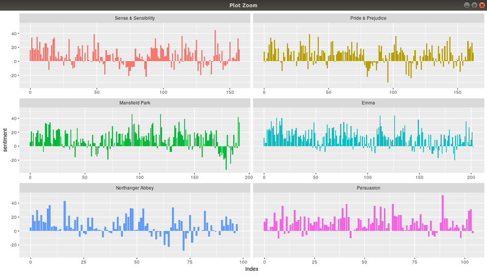
We could examine how sentiment changes throughout each novel

First, we need to find a sentiment value for each word in the austen_books() dataset:

We are going to use the Bing lexicon.

Using an inner_join() as explained above, we can have a sentiment value for each of the words in the austen_books() dataset that have been defined in the Bing lexicon:

janeaustensentiment <- tidy_books %>%
  inner_join(get_sentiments("bing")) %>%

Next, we count up how many positive and negative words there are in defined sections of each book:

We are going to define a section as a number of lines (80 lines in this case)

Small sections of text may not have enough words in them to get a good estimate of sentiment, while really large sections can wash out narrative structure. For these books, using 80 lines works well, but this can vary depending on individual texts, how long the lines were to start with, etc.

  %>%
  count(book, index = linenumber %/% 80, sentiment) %>%
Note how are we counting in defining sections of 80 lines using the count() command:

The count() command counts rows with equal values of the arguments specifies. In this case we want to count the number of rows with the same value of book, index (index = linenumber %/% 80), and sentiment.

The %/% operator does integer division (x %/% y is equivalent to floor(x/y))

So index = linenumber %/% 80 means that, for example, the first row (linenumber = 1) is going to have an index value of 0 (because 1 %/% 80 = 0). Thus:

linenumber = 1 --> index = 1 %/% 80 = 0'

linenumber = 79 --> index = 79 %/% 80 = 0'

linenumber = 80 --> index = 80 %/% 80 = 1'

linenumber = 159 --> index = 159 %/% 80 = 1'

linenumber = 160 --> index = 160 %/% 80 = 2'

...

This way, the count() command is counting how many positive and negative words there are every 80 lines.

Then we use the spread() command [from library(tidyr)] so that we have negative and positive sentiment in separate columns:

library(tidyr)

  %>%
  spread(sentiment, n, fill = 0) %>%

We lastly calculate a net sentiment (positive - negative):

  %>%
  mutate(sentiment = positive - negative)

Now we can plot these sentiment scores across the plot trajectory of each novel:

Notice that we are plotting against the index on the x-axis that keeps track of narrative time in sections of text.

library(ggplot2)

ggplot(janeaustensentiment, aes(index, sentiment, fill = book)) +
       geom_col(show.legend = FALSE) +
       facet_wrap(~book, ncol = 2, scales = "free_x")

Grouping the 5 previous scripts into a single script:

library(tidyr)
library(ggplot2)

janeaustensentiment <- tidy_books %>%
  inner_join(get_sentiments("bing")) %>%
  count(book, index = linenumber %/% 80, sentiment) %>% 
  spread(sentiment, n, fill = 0) %>%
  mutate(sentiment = positive - negative)

ggplot(janeaustensentiment, aes(index, sentiment, fill = book)) +
       geom_col(show.legend = FALSE) +
       facet_wrap(~book, ncol = 2, scales = "free_x")

Sentiment through the narratives of Jane Austen's novels

Comparing the Three Sentiment Dictionaries

pride_prejudice <- tidy_books %>%
  filter(book == "Pride & Prejudice")
pride_prejudice


afinn <- pride_prejudice %>%
  inner_join(get_sentiments("afinn")) %>%
  group_by(index = linenumber %/% 80) %>%
  summarise(sentiment = sum(score))   %>%
  mutate(method = "AFINN")

bing_and_nrc <- bind_rows(
  pride_prejudice %>%
    inner_join(get_sentiments("bing")) %>%
    mutate(method = "Bing et al."),
  pride_prejudice %>%
    inner_join(get_sentiments("nrc")   %>%
    filter(sentiment %in% c("positive","negative"))) %>%
    mutate(method = "NRC")) %>%
    count(method, index = linenumber   %/%
    80, sentiment) %>%
    spread(sentiment, n, fill = 0)     %>%
    mutate(sentiment = positive - negative)


bind_rows(afinn, bing_and_nrc) %>%
  ggplot(aes(index, sentiment, fill = method)) +
         geom_col(show.legend = FALSE) +
         facet_wrap(~method, ncol = 1, scales = "free_y")

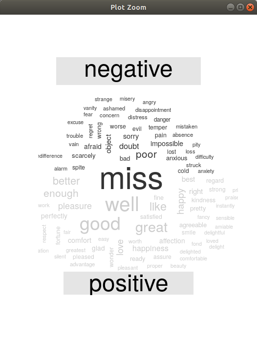
Comparing three sentiment lexicons using Pride and Prejudice

Most Common Positive and Negative Words

Wordclouds

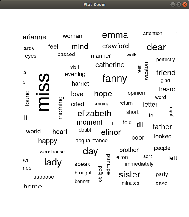
Using the wordcloud package, which uses base R graphics, let's look at the most common words in Jane Austen's works as a whole again, but this time as a wordcloud.

library(wordcloud)

tidy_books %>%
  anti_join(stop_words) %>%
  count(word) %>%
  with(wordcloud(word, n, max.words = 100))

The most common words in Jane Austen's novels

library(reshape2)

tidy_books %>%  
  inner_join(get_sentiments("bing")) %>%
  count(word, sentiment, sort = TRUE) %>%
  acast(word ~ sentiment, value.var = "n", fill = 0) %>%
  comparison.cloud(colors = c("gray20", "gray80"), max.words = 100)

Most common positive and negative words in Jane Austen's novels

Este tipo de graficos están presentando algunos problemas en mi instalación. No se grafican todas las palabras o no se despliegan de forma adecuada en la gráfica

Looking at Units Beyond Just Words

Unidades compuestas de varias palabras

Sometimes it is useful or necessary to look at different units of text. For example, some sentiment analysis algorithms look beyond only unigrams (i.e., single words) to try to understand the sentiment of a sentence as a whole. These algorithms try to understand that "I am not having a good day" is a sad sentence, not a happy one, because of negation.

Such sentiment analysis algorithms can be performed with the following R packages:

coreNLP (Arnold and Tilton 2016)
cleanNLP (Arnold 2016)
sentimentr (Rinker 2017)

For these, we may want to tokenize text into sentences, and it makes sense to use a new name for the output column in such a case.

Example 1:

PandP_sentences <- data_frame(text = prideprejudice) %>%
  unnest_tokens(sentence, text, token = "sentences")

Example 2:

austen_books()$text[45:83]
austen_books_sentences <- austen_books()[45:83,1:2] %>%
  unnest_tokens(sentence, text, token = "sentences")
austen_books_sentences

The sentence tokenizing does seem to have a bit of trouble with UTF-8 encoded text, especially with sections of dialogue; it does much better with punctuation in ASCII. One possibility, if this is important, is to try using iconv() with something like iconv(text, to = 'latin1') in a mutate statement before unnesting.

Another option in unnest_tokens() is to split into tokens using a regex pattern. We could use the following script, for example, to split the text of Jane Austen's novels into a data frame by chapter:

austen_chapters <- austen_books() %>%
  group_by(book) %>%
  unnest_tokens(chapter, text, token = "regex", pattern = "Chapter|CHAPTER [\\dIVXLC]") %>%
  ungroup()

austen_chapters %>%
  group_by(book) %>%
  summarise(chapters = n())

We have recovered the correct number of chapters in each novel (plus an "extra" row for each novel title). In the austen_chapters data frame, each row corresponds to one chapter.

Chapter 7 - Case Study - Comparing Twitter Archives

Machine Learning

What is Machine Learning

Al tratar de encontrar una definición para ML me di cuanta de que muchos expertos coinciden en que no hay una definición standard para ML.

En este post se explica bien la definición de ML: https://machinelearningmastery.com/what-is-machine-learning/

Estos vídeos también son excelentes para entender what ML is:

https://www.youtube.com/watch?v=f_uwKZIAeM0

https://www.youtube.com/watch?v=ukzFI9rgwfU

https://www.youtube.com/watch?v=WXHM_i-fgGo

https://www.coursera.org/lecture/machine-learning/what-is-machine-learning-Ujm7v

Una de las definiciones más citadas es la definición de Tom Mitchell. This author provides in his book Machine Learning a definition in the opening line of the preface:

Tom Mitchell

The field of machine learning is concerned with the question of how to construct computer programs that automatically improve with experience.

So, in short we can say that ML is about write computer programs that improve themselves.

Tom Mitchell also provides a more complex and formal definition:

Tom Mitchell

A computer program is said to learn from experience E with respect to some class of tasks T and performance measure P, if its performance at tasks in T, as measured by P, improves with experience E.

Don't let the definition of terms scare you off, this is a very useful formalism. It could be used as a design tool to help us think clearly about:

E: What data to collect.

T: What decisions the software needs to make.

P: How we will evaluate its results.

Suppose your email program watches which emails you do or do not mark as spam, and based on that learns how to better filter spam. In this case: https://www.coursera.org/lecture/machine-learning/what-is-machine-learning-Ujm7v

E: Watching you label emails as spam or not spam.

T: Classifying emails as spam or not spam.

P: The number (or fraction) of emails correctly classified as spam/not spam.

Types of Machine Learning

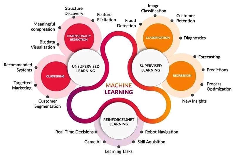
Supervised Learning

https://en.wikipedia.org/wiki/Supervised_learning

Supervised learning is the machine learning task of learning a function that maps an input to an output based on example input-output pairs.

In another words, it infers a function from labeled training data consisting of a set of training examples.

In supervised learning, each example is a pair consisting of an input object (typically a vector) and a desired output value (also called the supervisory signal).

A supervised learning algorithm analyzes the training data and produces an inferred function, which can be used for mapping new examples.

https://machinelearningmastery.com/supervised-and-unsupervised-machine-learning-algorithms/ The majority of practical machine learning uses supervised learning.

Supervised learning is when you have input variables (x) and an output variable (Y) and you use an algorithm to learn the mapping function from the input to the output.

Y = f(X)

The goal is to approximate the mapping function so well that when you have new input data (x) that you can predict the output variables (Y) for that data.

It is called supervised learning because the process of an algorithm learning from the training dataset can be thought of as a teacher supervising the learning process. We know the correct answers, the algorithm iteratively makes predictions on the training data and is corrected by the teacher. Learning stops when the algorithm achieves an acceptable level of performance.

https://www.datascience.com/blog/supervised-and-unsupervised-machine-learning-algorithms Supervised machine learning is the more commonly used between the two. It includes such algorithms as linear and logistic regression, multi-class classification, and support vector machines. Supervised learning is so named because the data scientist acts as a guide to teach the algorithm what conclusions it should come up with. It’s similar to the way a child might learn arithmetic from a teacher. Supervised learning requires that the algorithm’s possible outputs are already known and that the data used to train the algorithm is already labeled with correct answers. For example, a classification algorithm will learn to identify animals after being trained on a dataset of images that are properly labeled with the species of the animal and some identifying characteristics.

Supervised Classification

Supervised Classification with R: http://www.cmap.polytechnique.fr/~lepennec/R/Learning/Learning.html

Unsupervised Learning

Reinforcement Learning

Machine Learning Algorithms

Boosting

Gradient boosting

https://medium.com/mlreview/gradient-boosting-from-scratch-1e317ae4587d

https://freakonometrics.hypotheses.org/tag/gradient-boosting

https://en.wikipedia.org/wiki/Gradient_boosting

https://www.researchgate.net/publication/326379229_Exploring_the_clinical_features_of_narcolepsy_type_1_versus_narcolepsy_type_2_from_European_Narcolepsy_Network_database_with_machine_learning

http://arogozhnikov.github.io/2016/06/24/gradient_boosting_explained.html

Boosting is a machine learning ensemble meta-algorithm for primarily reducing bias, and also variance in supervised learning, and a family of machine learning algorithms that convert weak learners to strong ones. Boosting is based on the question posed by Kearns and Valiant (1988, 1989): "Can a set of weak learners create a single strong learner?" A weak learner is defined to be a classifier that is only slightly correlated with the true classification (it can label examples better than random guessing). In contrast, a strong learner is a classifier that is arbitrarily well-correlated with the true classification. https://en.wikipedia.org/wiki/Gradient_boosting

Gradient boosting is a machine learning technique for regression and classification problems, which produces a prediction model in the form of an ensemble of weak prediction models, typically decision trees. It builds the model in a stage-wise fashion like other boosting methods do, and it generalizes them by allowing optimization of an arbitrary differentiable loss function.

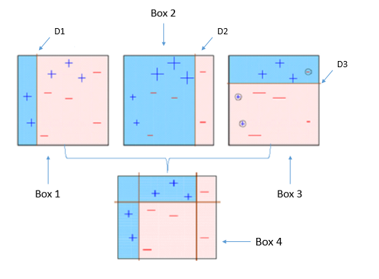
Boosting is a sequential process; i.e., trees are grown using the information from a previously grown tree one after the other. This process slowly learns from data and tries to improve its prediction in subsequent iterations. Let's look at a classic classification example:

Four classifiers (in 4 boxes), shown above, are trying hard to classify + and - classes as homogeneously as possible. Let's understand this picture well:

Box 1: The first classifier creates a vertical line (split) at D1. It says anything to the left of D1 is + and anything to the right of D1 is -. However, this classifier misclassifies three + points.

Box 2: The next classifier says don't worry I will correct your mistakes. Therefore, it gives more weight to the three + misclassified points (see bigger size of +) and creates a vertical line at D2. Again it says, anything to right of D2 is - and left is +. Still, it makes mistakes by incorrectly classifying three - points.

Box 3: The next classifier continues to bestow support. Again, it gives more weight to the three - misclassified points and creates a horizontal line at D3. Still, this classifier fails to classify the points (in circle) correctly.

Remember that each of these classifiers has a misclassification error associated with them.

Boxes 1,2, and 3 are weak classifiers. These classifiers will now be used to create a strong classifier Box 4.

Box 4: It is a weighted combination of the weak classifiers. As you can see, it does good job at classifying all the points correctly.

That's the basic idea behind boosting algorithms. The very next model capitalizes on the misclassification/error of previous model and tries to reduce it.

XGBoost in R

https://en.wikipedia.org/wiki/XGBoost

https://cran.r-project.org/web/packages/FeatureHashing/vignettes/SentimentAnalysis.html

https://www.hackerearth.com/practice/machine-learning/machine-learning-algorithms/beginners-tutorial-on-xgboost-parameter-tuning-r/tutorial/

https://xgboost.readthedocs.io/en/latest/R-package/xgboostPresentation.html

https://github.com/mammadhajili/tweet-sentiment-classification/blob/master/Report.pdf

https://datascienceplus.com/extreme-gradient-boosting-with-r/

https://www.analyticsvidhya.com/blog/2016/01/xgboost-algorithm-easy-steps/

https://www.r-bloggers.com/an-introduction-to-xgboost-r-package/

https://www.kaggle.com/rtatman/machine-learning-with-xgboost-in-r

https://rpubs.com/flyingdisc/practical-machine-learning-xgboost

https://www.youtube.com/watch?v=woVTNwRrFHE

Artificial neural network

https://en.wikipedia.org/wiki/Artificial_neural_network

Natural Language Processing - NLP

Sentiment Analysis

Sentiment Analysis with R

https://medium.com/datadriveninvestor/twitter-sentiment-analysis-of-movie-reviews-using-machine-learning-techniques-23d4724e7b05

https://github.com/Twitter-Sentiment-Analysis/R

https://github.com/jayskhatri/Sentiment-Analysis-of-Twitter

https://hackernoon.com/text-processing-and-sentiment-analysis-of-twitter-data-22ff5e51e14c

http://tabvizexplorer.com/sentiment-analysis-using-r-and-twitter/

https://analyzecore.com/2017/02/08/twitter-sentiment-analysis-doc2vec/

https://github.com/rbhatia46/Twitter-Sentiment-Analysis-Web

http://dataaspirant.com/2018/03/22/twitter-sentiment-analysis-using-r/

https://www.r-bloggers.com/twitter-sentiment-analysis-with-r/

Training a machine to classify tweets according to sentiment

https://rpubs.com/imtiazbdsrpubs/236087

# https://rpubs.com/imtiazbdsrpubs/236087

library(twitteR)
library(base64enc)
library(tm)
library(RTextTools)
library(qdapRegex)
library(dplyr)



# -------------------------------------------------------------------------- -
# ���� Authentication through api to get the data ----
# -------------------------------------------------------------------------- -
consumer_key<-'EyViljD4yD3e3iNEnRvYnJRe8'
consumer_secret<-'mN8vjKR0oqDCReCr77Xx81BK0epQZ6MiPggPtDzYXDpxDzM5vu'
access_token<-'3065887431-u1mtPeXAOehZKuuhTCswbstoRZdadYghIrBiFHS'
access_secret<-'afNNt3hdZZ5MCFOEPC4tuq3dW3NPzU403ABPXHOHKtFFn'

# After this line of command type 1 for selection as Yes:
setup_twitter_oauth(consumer_key, consumer_secret, access_token, access_secret)
## [1] "Using direct authentication"




# -------------------------------------------------------------------------- -
# ���� Getting Tweets from the api and storing the data based on hashtags ----
# -------------------------------------------------------------------------- -
hashtags = c('#ClimateChange', '#Trump', '#Demonetization', '#Kejriwal', '#Technology')
totalTweets= list()
for (hashtag in hashtags){
  tweets = searchTwitter(hashtag, n=20 )       # Search fot tweets (n specify the number of tweets)
  tweets = twListToDF(tweets)                  # Convert from list to dataframe
  
  tweets <- tweets  %>%                        # Adding a column to specify which hashtag the tweet come from
    mutate(hashtag = hashtag)
  
  tweets.df = tweets[,1]                       # Assign tweets for cleaning

  tweets.df = gsub("(RT|via)((?:\\b\\W*@\\w+)+)", "", tweets.df);head(tweets.df) 
  
  tweets.df  = gsub("@\\w+", "", tweets.df);head(tweets.df)         # Regex for removing @user
  tweets.df  = gsub("[[:punct:]]", "", tweets.df);head(tweets.df)   # Regex for removing punctuation mark
  tweets.df  = gsub("[[:digit:]]", "", tweets.df);head(tweets.df)   # Regex for removing numbers
  tweets.df  = gsub("http\\w+", "", tweets.df);head(tweets.df)      # Regex for removing links
  tweets.df  = gsub("\n", " ", tweets.df);head(tweets.df)           # Regex for removing new line (\n)
  tweets.df  = gsub("[ \t]{2,}", " ", tweets.df);head(tweets.df)    # Regex for removing two blank space
  tweets.df  = gsub("[^[:alnum:]///' ]", " ", tweets.df)            # Keep only alpha numeric 
  tweets.df  = iconv(tweets.df, "latin1", "ASCII", sub="")          # Keep only ASCII characters
  tweets.df  = gsub("^\\s+|\\s+$", "", tweets.df);head(tweets.df)   # Remove leading and trailing white space
  tweets[,1] = tweets.df                                            # Save in Data frame
  totalTweets[[paste0(gsub('#','',hashtag))]]=tweets
}

# Combining all the tweets into a single corpus
HashTagTweetsCombined = do.call("rbind", totalTweets)

dim(HashTagTweetsCombined)
str(HashTagTweetsCombined)

str(HashTagTweetsCombined)




# -------------------------------------------------------------------------- -
# ���� Text preprocessing using the qdap regex package ----
# -------------------------------------------------------------------------- -
HashTagTweetsCombined$text=sapply(HashTagTweetsCombined$text,rm_url,pattern=pastex("@rm_twitter_url", "@rm_url"))  # Cleaning the text: Removing URL's
HashTagTweetsCombined$text=sapply(HashTagTweetsCombined$text,rm_email)      # Removing emails from the tweet text(rm_email removes all the patterns which has @)
HashTagTweetsCombined$text=sapply(HashTagTweetsCombined$text,rm_tag)        # Removes user hash tags from the tweet text
HashTagTweetsCombined$text=sapply(HashTagTweetsCombined$text,rm_number)     # Removes numbers from the text
HashTagTweetsCombined$text=sapply(HashTagTweetsCombined$text,rm_non_ascii)  # Removes non ascii characters
HashTagTweetsCombined$text=sapply(HashTagTweetsCombined$text,rm_white)      # Removes extra white spaces
HashTagTweetsCombined$text=sapply(HashTagTweetsCombined$text,rm_date)       # Removes dates from the text




# -------------------------------------------------------------------------- -
# ���� Manually label the polarity of the tweets into -neutral- -positive- and -negative- sentiments ----
# -------------------------------------------------------------------------- -
# Storing the file in local location so as to manually label the polarity
# write.table(HashTagTweetsCombined,"/home/anapaula/HashTagTweetsCombined.csv", append=T, row.names=F, col.names=T,  sep=",")

# Reloading the file again after manually labelling
HashTagTweetsCombined=read.csv("/home/anapaula/HashTagTweetsCombined.csv")
# HashTagTweetsCombined$sentiment=factor(HashTagTweetsCombined$sentiment)




# -------------------------------------------------------------------------- -
# ���� Splitting the data into train and test data ----
# -------------------------------------------------------------------------- -
data <- HashTagTweetsCombined  %>%          # Taking just the columns we are interested in (slicing the data)
  select(text, sentiment, hashtag)

set.seed(16102016)                          # To fix the sample 

# Randomly Taking the 70% of the rows (70% records will be used for training  sampling without replacement. The remaining 30% will be used for testing)
samp_id = sample(1:nrow(data),              # do ?sample to examine the sample() func
                 round(nrow(data)*.70),
                 replace = F)
train = data[samp_id,]                      # 70% of training data set, examine struc of samp_id obj
test  = data[-samp_id,]                     # remaining 30% of training data set
dim(train) ; dim(test)

# Join the data sets
train.data = rbind(train,test)




# -------------------------------------------------------------------------- -
# ���� Text processing ----
# -------------------------------------------------------------------------- -
train.data$text = tolower(train.data$text)  # Convert to lower case
text = train.data$text                      # Taking just the text column
text = removePunctuation(text)              # Remove punctuation marks
text = removeNumbers(text)                  # Remove numbers
text = stripWhitespace(text)                # Remove blank space




# -------------------------------------------------------------------------- -
# ���� Creating the document term matrix ----
# -------------------------------------------------------------------------- -
# https://en.wikipedia.org/wiki/Document-term_matrix

cor  = Corpus(VectorSource(text))           # Create text corpus
dtm  = DocumentTermMatrix(cor,              # Craete DTM
                          control = list(weighting =
                                          function(x)
                                            weightTfIdf(x, normalize = F)))  # IDF weighing
dim(dtm)


# sorts a sparse matrix in triplet format (i,j,v) first by i, then by j  (https://groups.google.com/forum/#!topic/rtexttools-help/VILrGoRpRrU)
# Args:
#   working.dtm: a sparse matrix in i,j,v format using $i $j and $v respectively. Any other variables that may exist in the sparse matrix are not operated on, and will be returned as-is.
# Returns:
#   A sparse matrix sorted by i, then by j.
ResortDtm <- function(working.dtm) {
  working.df <- data.frame(i = working.dtm$i, j = working.dtm$j, v = working.dtm$v)  # create a data frame comprised of i,j,v values from the sparse matrix passed in.
  working.df <- working.df[order(working.df$i, working.df$j), ]                      # sort the data frame first by i, then by j.
  working.dtm$i <- working.df$i                                                      # reassign the sparse matrix' i values with the i values from the sorted data frame.
  working.dtm$j <- working.df$j                                                      # ditto for j values.
  working.dtm$v <- working.df$v                                                      # ditto for v values.
  return(working.dtm)                                                                # pass back the (now sorted) data frame.
}

dtm <- ResortDtm(dtm)


# Coded labels
training_codes = train.data$sentiment




# -------------------------------------------------------------------------- -
# ���� Creating the model: Testing different models and choosing the best model ----
# -------------------------------------------------------------------------- -
# After many iterations and testing with models like RF, TREE, Bagging, maxent, and slda, we found that GLMNET is giving higher accuracy

# Creates a 'container' obj for training, classifying, and analyzing docs
container <- create_container(dtm,
                              t(training_codes),                             # Labels or the Y variable / outcome we want to train on
                              trainSize = 1:nrow(train),
                              testSize  = (nrow(train)+1):nrow(train.data),
                              virgin    = FALSE)                             # Whether to treat the classification data as 'virgin' data or not
                                                                             # If virgin = TRUE, then machine won;t borrow from prior datasets
str(container)                                                               # View struc of the container obj; is a list of training n test data


# Creating the model
models  <- train_models(container,                     # ?train_models; makes a model object using the specified algorithms.
                        algorithms=c("GLMNET"))        # "MAXENT","SVM","GLMNET","SLDA","TREE","BAGGING","BOOSTING","RF"




# -------------------------------------------------------------------------- -
# ���� Makes predictions from a train_models() object ----
# -------------------------------------------------------------------------- -
results <- classify_models(container, models)
head(results)




# -------------------------------------------------------------------------- -
# ���� Determining the accuracy of prediction results ----
# -------------------------------------------------------------------------- -
# Building a confusion matrix
out = data.frame(model_sentiment  = results$GLMNET_LABEL,                                    # Rounded probability == model's prediction of Y
                 model_prob       = results$GLMNET_PROB,
                 actual_sentiment = train.data$sentiment[(nrow(train)+1):nrow(train.data)])  # Actual value of Y

dim(out); head(out);

summary(out)                                       # How many 0s and 1s were there anyway?
(z = as.matrix(table(out[,1], out[,3])))           # Display the confusion matrix.
(pct = round(((z[1,1] + z[2,2])/sum(z))*100, 2))   # Prediction accuracy in % terms

Social Media Sentiment Analysis

https://www.dezyre.com/article/top-10-machine-learning-projects-for-beginners/397

https://elitedatascience.com/machine-learning-projects-for-beginners#social-media

https://en.wikipedia.org/wiki/Sentiment_analysis

https://en.wikipedia.org/wiki/Social_media_mining

Sentiment analysis, also known as opinion mining, opinion extraction, sentiment mining or subjectivity analysis, is the process of analyzing a piece of online writing (social media mentions, blog posts, news sites, or any other piece) expresses positive, negative, or neutral attitude. https://brand24.com/blog/twitter-sentiment-analysis/

Motivation

Social media has almost become synonymous with «big data» due to the sheer amount of user-generated content.

Mining this rich data can prove unprecedented ways to keep a pulse on opinions, trends, and public sentiment (Facebook, Twitter, YouTube, WeChat...)

Social media data will become even more relevant for marketing, branding, and business as a whole.

As you can see, Data Analysis (Machine learning) for this kind of researches is a tool that will become more and more important in the coming years.

Methodology

Mining Social Media data

The first part of the project will be Mining Social Media data

To start the project we first need to choose where we are going to get the data from. I have seen in many sources that to start working on it, Twitter is the classic entry point for practicing. Here you can see a tutorial about how to Mining Twitter Data with Python : https://marcobonzanini.com/2015/03/02/mining-twitter-data-with-python-part-1/

=Twitter Data Mining=

https://www.toptal.com/python/twitter-data-mining-using-python

https://marcobonzanini.com/2015/03/02/mining-twitter-data-with-python-part-1/

Why Twitter data?

Twitter is a gold mine of data. Unlike other social platforms, almost every user’s tweets are completely public and pullable. This is a huge plus if you’re trying to get a large amount of data to run analytics on. Twitter data is also pretty specific. Twitter’s API allows you to do complex queries like pulling every tweet about a certain topic within the last twenty minutes, or pull a certain user’s non-retweeted tweets.

A simple application of this could be analyzing how your company is received in the general public. You could collect the last 2,000 tweets that mention your company (or any term you like), and run a sentiment analysis algorithm over it.

We can also target users that specifically live in a certain location, which is known as spatial data. Another application of this could be to map the areas on the globe where your company has been mentioned the most.

As you can see, Twitter data can be a large door into the insights of the general public, and how they receive a topic. That, combined with the openness and the generous rate limiting of Twitter’s API, can produce powerful results.

Twitter Developer Account:

In order to use Twitter’s API, we have to create a developer account on the Twitter apps site.

Log in or make a Twitter account at https://apps.twitter.com/

As of July 2018, you must apply for a Twitter developer account and be approved before you may create new apps. Once approved, you will be able to create new apps from developer.twitter.com.

Home Twitter Developer Account: https://developer.twitter.com/

Tutorials:https://developer.twitter.com/en/docs/tutorials

Docs: https://developer.twitter.com/en/docs

How to Register a Twitter App: https://iag.me/socialmedia/how-to-create-a-twitter-app-in-8-easy-steps/

Storing the data

Secondly, we will need to store the data

Analyzing the data

The third part of the project will be the analysis of the data. Here is where Machine learning will be implement.

In this part we first need to decide what we want to analyze. There are many examples:

Example 1 - Business: companies use opinion mining tools to find out what consumers think of their product, service, brand, marketing campaigns or competitors.

Example 2 - Public actions: opinion analysis is used to analyze online reactions to social and cultural phenomena, for example, the premiere episode of the Game of Thrones, or Oscars.

Example 3 - Politics: In politics, sentiment analysis is used to keep track of society’s opinions on the government, politicians, statements, policy changes, or event to predict results of the election.

Here the link to a nice article I found «This article describes the techniques that effectively analyzed Twitter Trend Topics to predict, as a sample test case, regional voting patterns in the 2014 Brazilian presidential election» : https://www.toptal.com/data-science/social-network-data-mining-for-predictive-analysis

In essence, this guy analyses Twitter data for the days prior to the election and got this map:

Example 4 - Health: I found, for example, this topic that I think is really interesting: Using Twitter Data and Sentiment Analysis to Study Diseases Dynamics. In this work, we extract information about diseases from Twitter with spatiotemporal constraints, i.e. considering a specific geographic area during a given period. We show our first results for a monitoring tool that allow to study the dynamic of diseases https://www.researchgate.net/publication

Plotting the data

If we decide to plot Geographical trends of data, we could present the data using JavaScript like this (Click into the regions and countries): http://perso.sinfronteras.ws/1-archivos/javascript_maps-ammap/continentes.html

Some remarks

It will be up to us (as a team) to determine what we want to analyses. However, we don't need to decide RIGHT NOW what we are going to analyses. A big part of the methodology can be done without knowing what we are going to analyses. We have enough time to think about a nice case study...

Another important feature of this work if that we can do it as complex as we want. We could start with something simple like: Determining the most relevant Twitter topic in a geographic area (Dublin for example) during a given period; and following a similar methodology, implement some more complex or relevant analysis like that one about Study Diseases Dynamics; or whichever we decide as a team.

Some references

https://brand24.com/blog/twitter-sentiment-analysis/

https://elitedatascience.com/machine-learning-projects-for-beginners#social-media

https://www.dezyre.com/article/top-10-machine-learning-projects-for-beginners/397

https://www.researchgate.net/publication/283634023_Using_Twitter_Data_and_Sentiment_Analysis_to_Study_Diseases_Dynamics

https://www.toptal.com/data-science/social-network-data-mining-for-predictive-analysis

Text Classification

https://monkeylearn.com/text-classification/

Text classification is the process of assigning tags or categories to text according to its content. It’s one of the fundamental tasks in Natural Language Processing (NLP) with broad applications such as sentiment analysis, topic labeling, spam detection, and intent detection.

Unstructured data in the form of text is everywhere: emails, chats, web pages, social media, support tickets, survey responses, and more. Text can be an extremely rich source of information, but extracting insights from it can be hard and time-consuming due to its unstructured nature. Businesses are turning to text classification for structuring text in a fast and cost-efficient way to enhance decision-making and automate processes.

But, what is text classification? How does text classification work? What are the algorithms used for classifying text? What are the most common business applications?

Text classification (a.k.a. text categorization or text tagging) is the task of assigning a set of predefined categories to free-text. Text classifiers can be used to organize, structure, and categorize pretty much anything. For example, new articles can be organized by topics, support tickets can be organized by urgency, chat conversations can be organized by language, brand mentions can be organized by sentiment, and so on.

As an example, take a look at the following text below:

"The user interface is quite straightforward and easy to use."

A classifier can take this text as an input, analyze its content, and then and automatically assign relevant tags, such as UI and Easy To Use that represent this text:

There are many approaches to automatic text classification, which can be grouped into three different types of systems:

Rule-based systems
Machine Learning based systems
Hybrid systems

Machine Learning Based Systems

Instead of relying on manually crafted rules, text classification with machine learning learns to make classifications based on past observations. By using pre-labeled examples as training data, a machine learning algorithm can learn the different associations between pieces of text and that a particular output (i.e. tags) is expected for a particular input (i.e. text).

The first step towards training a classifier with machine learning is feature extraction: a method is used to transform each text into a numerical representation in the form of a vector. One of the most frequently used approaches is bag of words, where a vector represents the frequency of a word in a predefined dictionary of words.

For example, if we have defined our dictionary to have the following words {This, is, the, not, awesome, bad, basketball}, and we wanted to vectorize the text “This is awesome”, we would have the following vector representation of that text: (1, 1, 0, 0, 1, 0, 0).

Then, the machine learning algorithm is fed with training data that consists of pairs of feature sets (vectors for each text example) and tags (e.g. sports, politics) to produce a classification model:

Once it’s trained with enough training samples, the machine learning model can begin to make accurate predictions. The same feature extractor is used to transform unseen text to feature sets which can be fed into the classification model to get predictions on tags (e.g. sports, politics):

Text Classification Algorithms

Some of the most popular machine learning algorithms for creating text classification models include the naive bayes family of algorithms, support vector machines, and deep learning.

Naive Bayes

Support vector machines

Deep learning

Fake news detection

Supervised Machine Learning for Fake News Detection

Fake news Challenge

http://www.fakenewschallenge.org/

Exploring how artificial intelligence technologies could be leveraged to combat fake news.

Formal Definition

Input: A headline and a body text - either from the same news article or from two different articles.

Output: Classify the stance of the body text relative to the claim made in the headline into one of four categories:
- Agrees: The body text agrees with the headline.
- Disagrees: The body text disagrees with the headline.
- Discusses: The body text discuss the same topic as the headline, but does not take a position
- Unrelated: The body text discusses a different topic than the headline

Stance Detection dataset for FNC1

https://github.com/FakeNewsChallenge/fnc-1

Winner teams

First place - Team SOLAT in the SWEN https://github.com/Cisco-Talos/fnc-1
The data provided is (headline, body, stance) instances, where stance is one of {unrelated, discuss, agree, disagree}. The dataset is provided as two CSVs:

train_bodies.csv : This file contains the body text of articles (the articleBody column) with corresponding IDs (Body ID)

train_stances.csv : This file contains the labeled stances (the Stance column) for pairs of article headlines (Headline) and article bodies (Body ID, referring to entries in train_bodies.csv).

Distribution of the data

The distribution of Stance classes in train_stances.csv is as follows:

rows	unrelated	discuss	agree	disagree
49972	0.73131	0.17828	0.0736012	0.0168094

Paper: Fake news detection on social media - A data mining perspective

Paper: Automatic Detection of Fake News in Social Media using Contextual Information

https://brage.bibsys.no/xmlui/bitstream/handle/11250/2559124/18038_FULLTEXT.pdf?sequence=1&isAllowed=y

Linguistic approach

The linguistic or textual approach to detecting false information involves using techniques that analyzes frequency, usage, and patterns in the text. Using this gives the ability to find similarities that comply to usage that is known in types of text, such as for fake news, which have a language that is similar to satire and will contain more emotional and an easier language than articles have on the same topic.

Support VectorMachines A support vector machine(SVM) is a classifier that works by separating a hyperplane(n-dimensional space) containing input. It is based on statistical learning theory[59]. Given labeled training data, the algorithm outputs an optimal hyperplane which classifies new examples. The optimal hyperplane is calculated by finding the divider that minimizes the noise sensitivity andmaximizes the generalization
Naive Bayes Naive Bayes is a family of linear classifiers that works by using mutually independent features in a dataset for classification[46]. It is known for being easy to implement, being robust, fast and accurate. They are widely used for classification tasks, such as diagnosis of diseases and spam filtering in E-mail.
Term frequency inverse document frequency Term frequency-inverse document frequency(TF-IDF) is a weight value often used in information retrieval and gives a statistical measure to evaluate the importance of a word in a document collection or a corpus. Basically, the importance of a word increases proportionally with how many times it appears in a document, but is offset by the frequency of the word in the collection or corpus. Thus a word that appears all the time will have a low impact score, while other less used words will have a greater value associated with them[28]
N-grams
Sentiment analysis

Contextual approach

Contextual approaches incorporate most of the information that is not text. This includes data about users, such as comments, likes, re-tweets, shares and so on. It can also be information regarding the origin, both as who created it and where it was first published. This kind of information has a more predictive approach then linguistic, where you can be more deterministic. The contextual clues give a good indication of how the information is being used, and based on this assumptions can be made.

This approach relies on structured data to be able to make the assumptions, and because of that the usage area is for now limited to Social Media, because of the amount of information that is made public there. You have access to publishers, reactions, origin, shares and even age of the posts.

In addition to this, contextual systems are most often used to increase the quality of existing information and augment linguistic systems, by giving more information to work on for these systems, being reputation, trust metrics or other ways of giving indicators on whether the information is statistically leaning towards being fake or not.

Below a series of contextual methods are presented. They are a collection of state of the art methods and old, proven methods.

Logistic regression
Crowdsourcing algorithms
Network analysis
Trust Networks
Trust Metrics
Content-driven reputation system
Knowledge Graphs

Paper: Fake News Detection using Machine Learning

https://www.pantechsolutions.net/machine-learning-projects/fake-news-detection-using-machine-learning

Blog: I trained fake news detection AI with >95% accuracy and almost went crazy

https://towardsdatascience.com/i-trained-fake-news-detection-ai-with-95-accuracy-and-almost-went-crazy-d10589aa57c

Collecting data from Twitter using R

install.packages("twitteR")
library(twitteR)

consumer_key<-'EyViljD4yD3e3iNEnRvYnJRe8'
consumer_secret<-'mN8vjKR0oqDCReCr77Xx81BK0epQZ6MiPggPtDzYXDpxDzM5vu'
access_token<-'3065887431-u1mtPeXAOehZKuuhTCswbstoRZdadYghIrBiFHS'
access_secret<-'afNNt3hdZZ5MCFOEPC4tuq3dW3NPzU403ABPXHOHKtFFn'

setup_twitter_oauth(consumer_key, consumer_secret, access_token, access_secret)

# terms <- c("iphonex", "iPhonex", "iphoneX", "iPhoneX", "iphone10", "iPhone10","iphone x", "iPhone x", "iphone X", "iPhone X", "iphone 10", "iPhone 10", "#iphonex", "#iPhonex", "#iphoneX", "#iPhoneX", "#iphone10", "#iPhone10")
terms <- c("Football")

terms_search <- paste(terms, collapse = " OR ")

iphonex <- searchTwitter(terms_search, n=1000, lang="ur")
iphonex <- twListToDF(iphonex)
write.table(iphonex,"/home/anapaula/iphonex.csv", append=T, row.names=F, col.names=T,  sep=",")

Some important concepts

Confusion matrix

https://www.dataschool.io/simple-guide-to-confusion-matrix-terminology/

Programming and Applications for Data Science

Python for Data Science

R Programming

RTextTools - A Supervised Learning Package for Text Classification

https://journal.r-project.org/archive/2013/RJ-2013-001/RJ-2013-001.pdf

http://www.rtexttools.com/

https://cran.r-project.org/web/packages/RTextTools/index.html

The train_model() function takes each algorithm, one by one, to produce an object passable to classify_model().

A convenience train_models() function trains all models at once by passing in a vector of model requests. The syntax below demonstrates model creation for all nine algorithms:


Algorithms	Author	From package	Keyword
General linearized models	Friedman et al., 2010	glmnet	GLMNET*
Support vector machine	Meyer et al., 2012	e1071	SVM*
Maximum entropy	Jurka, 2012	maxent	MAXENT*
Classification or regression tree	Ripley., 2012	tree	TREE
Random forest	Liawand Wiener, 2002	randomForest	RF
Boosting	Tuszynski, 2012	caTools	BOOSTING
Neural networks	Venables and Ripley, 2002	nnet	NNET
Bagging	Peters and Hothorn, 2012	ipred	BAGGING**
Scaled linear discriminant analysis	Peters and Hothorn, 2012	ipred	SLDA**
* Low-memory algorithm ** Very high-memory algorithm

GLMNET <- train_model(container,"GLMNET")