|
|
| Line 3: |
Line 3: |
| | |+ | | |+ |
| | |- | | |- |
| − | ! style="vertical-align:top;" |<h5 style="text-align:left; vertical-align:top">Confusion Matrix or Coincidence Matrix</h5> | + | ! colspan="3" style="vertical-align:top;" |Regression Error: |
| − | |[[File:Regression_errors.png|300px|center|]] | + | |
| − | |
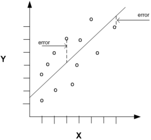
| + | The evaluation of regression models involves calculation on the errors (also known as residuals or innovations). |
| − | {| class="wikitable" style="center" | + | |
| − | |+
| + | Errors are the differences between the predicted values, represented as <math>\hat{y}</math> and the actual values, denoted <math>y</math>. |
| | + | {| |
| | + | ![[File:Regression_errors.png|300px|center|link=Special:FilePath/Regression_errors.png]] |
| | + | ! |
| | + | {| class="wikitable" |
| | !<math>y</math> | | !<math>y</math> |
| | !<math>\hat{y}</math> | | !<math>\hat{y}</math> |
| Line 31: |
Line 35: |
| | |10 | | |10 |
| | |2.5 | | |2.5 |
| | + | |} |
| | |} | | |} |
| | |- | | |- |
| Line 152: |
Line 157: |
| | </div> | | </div> |
| | </div> | | </div> |
| − | |-
| |
| − | ! style="vertical-align:top;" |<h5 style="text-align:left; vertical-align:top">Matthews Correlation Coefficient</h5>
| |
| − | |
| |
| − | <div class="mw-collapsible mw-collapsed" data-expandtext="+/-" data-collapsetext="+/-">
| |
| − | The F1-Score is adequate as a metric when precision and recall are considered equally important, or when the relative weighting between the two can be determined non-arbitrarily.
| |
| − |
| |
| − | An alternative for cases where that does not apply is the '''Matthews Correlation Coefficient'''. It returns a value in the interval <math>[-1,+1]</math>, where -1 suggests total disagreement between predicted values and actual values, 0 is indicative that any agreement is the product of random chance and +1 suggests perfect prediction.
| |
| − | <div class="mw-collapsible-content">
| |
| − | <br />
| |
| − | So, if the value is -1, every value that is true will be predicted as false and everyone that is false will be predicted as true. If the value is 1, every value that is true will be predicted as such and every value that is false will be predicted as such.
| |
| − |
| |
| − |
| |
| − | Unlike any of the metrics we have seen in previous slides, the Matthews Correlation coefficient takes into account all four categories in the confusion matrix.
| |
| − | </div>
| |
| − | </div>
| |
| − | |
| |
| − | <div class="mw-collapsible mw-collapsed" data-expandtext="+/-" data-collapsetext="+/-">
| |
| − | <math>
| |
| − | MCC = \frac{TP \times TN - FP \times FN}{\sqrt{(TP + FP) \times (TP + FN) \times (TN + FP) \times (TN + FN)}}
| |
| − | </math>
| |
| − | <div class="mw-collapsible-content">
| |
| − | <br />
| |
| − | <math>
| |
| − | MCC = \frac{1728 - 128}{\sqrt{88 \times 80 \times 40 \times 32}} = 0.5330
| |
| − | </math>
| |
| − | </div>
| |
| − | </div>
| |
| − | |-
| |
| − | ! style="vertical-align:top;" |<h5 style="text-align:left; vertical-align:top">Cohen's Kappa</h5>
| |
| − | |
| |
| − | <div class="mw-collapsible mw-collapsed" data-expandtext="+/-" data-collapsetext="+/-">
| |
| − | Cohen's Kappa is a measure of the amount of agreement between two raters classifying N items into C mutually-exclusive categories.
| |
| − |
| |
| − |
| |
| − | It is defined by the equation given below, where <math>\rho_0</math> is the observed agreement between raters and <math>\rho_e</math> is the hypothetical agreement that would be expected to occur by random chance.
| |
| − |
| |
| − |
| |
| − | Landis and Koch (1977) suggest an interpretation of the magnitude of the results as follows:
| |
| − |
| |
| − | <math>
| |
| − | \begin{array}{lcl}
| |
| − | 0 & = & \text{agreement equivalent to chance} \\
| |
| − | 0.10 - 0.20 & = & \text{slight agreement} \\
| |
| − | 0.21 - 0.40 & = & \text{fair agreement} \\
| |
| − | 0.41 - 0.60 & = & \text{moderate agreement} \\
| |
| − | 0.61 - 0.80 & = & \text{substantial agreement} \\
| |
| − | 0.81 - 0.99 & = & \text{near perfect agreement} \\
| |
| − | 1 & = & \text{perfect agreement} \\
| |
| − | \end{array}
| |
| − | </math>
| |
| − | <div class="mw-collapsible-content">
| |
| − | <br />
| |
| − | ...
| |
| − | </div>
| |
| − | </div>
| |
| − | |
| |
| − | <div class="mw-collapsible mw-collapsed" data-expandtext="+/-" data-collapsetext="+/-">
| |
| − | <math>K = 1 - \frac{1 - \rho_0}{1 - \rho_e}</math>
| |
| − | <div class="mw-collapsible-content">
| |
| − | <br />
| |
| − | *'''Calculate <math>\rho_0</math>'''<blockquote>The agreement on the positive class is 72 instances and on the negative class is 24 instances. So the agreement is 96 instances out of a total of 120<math>\rho_0 = \frac{96}{120} = 0.7</math> Note this is the same as the accuracy
| |
| − |
| |
| − | *'''Calculate the probability of random agreement on the «positive» class:'''
| |
| − |
| |
| − | <blockquote>The probability that both actual and predicted would agree on the positive class at random is the proportion of the total the positive class makes up for each of actual and predicted.
| |
| − |
| |
| − | For the actual class, this is:
| |
| − |
| |
| − | <math>\frac{(72 + 8)}{120} = 0.6666</math>
| |
| − |
| |
| − | For the predicted class this is:
| |
| − |
| |
| − | <math>\frac{(72 + 16)}{120} = 0.7333</math>
| |
| − |
| |
| − | The total probability that both actual and predicted will randomly agree on the positive class is <math>0.6666 \times 0.7333 = 0.4888</math></blockquote>
| |
| − |
| |
| − | *'''Calculate the probability of random agreement on the «negative» class:'''
| |
| − |
| |
| − | <blockquote>The probability that both actual and predicted would agree on the negative class at random is the proportion of the total the negative class makes up for each of actual and predicted.
| |
| − |
| |
| − | For the actual class, this is
| |
| − |
| |
| − | <math>\frac{(16 + 24)}{120} = 0.3333</math>
| |
| − |
| |
| − | For the predicted class this is
| |
| − |
| |
| − | <math>\frac{(8 + 24)}{120} = 0.2666</math>
| |
| − |
| |
| − | The total probability that both actual and predicted will randomly agree on the negative class is <math>0.3333 \times 0.2666 = 0.0888</math></blockquote>
| |
| − |
| |
| − | *'''Calculate <math>\rho_e</math>'''
| |
| − |
| |
| − | <blockquote>The probability <math>\rho_e</math> is simply the sum of the results of the calculations previously calculated:
| |
| − |
| |
| − | <math>\rho_e = 0.4888 + 0.0888 = 0.5776</math></blockquote>
| |
| − |
| |
| − | *'''Calculate kappa:'''
| |
| − |
| |
| − | <blockquote>
| |
| − | <math>
| |
| − | K = 1 - \frac{1 - \rho_0}{1- \rho_e}</math> <math>= 1 - \frac{1 - 0.7}{1 - 0.5776} = 0.2898
| |
| − | </math>
| |
| − |
| |
| − | This indicates a 'fair agreement' according to the scale suggested by Lanis and Koch (1977)
| |
| − | </blockquote>
| |
| − | </div>
| |
| − | </div>
| |
| − | |-
| |
| − | ! style="vertical-align:top;" |<h5 style="text-align:left; vertical-align:top">The receiver Operator Characteristic Curve</h5>
| |
| − | |
| |
| − | <div class="mw-collapsible mw-collapsed" data-expandtext="+/-" data-collapsetext="+/-">
| |
| − | The Receiver Operating Characteristic Curve has its origins in radio transmission, but in this context is a method to visually evaluate the performance of a classifier. It is a 2D trap with the true positive rate on the x-axis and the false positive rate on the y-axis.
| |
| − |
| |
| − |
| |
| − | '''There are 4 keys points on a ROC curve:'''
| |
| − |
| |
| − | * (0,0): classifier doesn't do anything
| |
| − | * (1,1): classifier always predict true
| |
| − | * (0,1): perfect classifier that never issues a false positive
| |
| − | * Line y = x: random classification (coin toss); the standards base line
| |
| − |
| |
| − |
| |
| − | '''Any classifier is:'''
| |
| − |
| |
| − | * better the closer it is to the point (0,1)
| |
| − | * conservative if it is on the left-hand side of the graph
| |
| − | * liberal if they are in on the upper right of the graph
| |
| − | <div class="mw-collapsible-content">
| |
| − | <br />
| |
| − | '''To create a ROC curve we do the following:'''
| |
| − |
| |
| − | * Rank the prediction of ta classifier by confidence in (or probability of) correct classification
| |
| − | * Order them (highest first)
| |
| − | * Plot each prediction's impact on the true positive rate and false-positive rate.
| |
| − |
| |
| − |
| |
| − | Classifiers are considered conservative if they make positive classifications in the presence of strong evidence, so they make fewer false-positive errors, typically at the cost of low true positive rates.
| |
| − |
| |
| − | Classifiers are considered liberal if they make positive classifications with weak evidence so they classify nearly all positives correctly, typically at the cost of high false-positive rates.
| |
| − |
| |
| − |
| |
| − | May real-world data sets are dominated by negative instances. The left-hand side of the ROC curve is, therefore, more interesting.
| |
| − | </div>
| |
| − | </div>
| |
| − | |
| |
| − | [[File:ROC_curve.png|center|350px]]
| |
| − | |-
| |
| − | !style="vertical-align:top;" |<h5 style="text-align:left; vertical-align:top">The Area Under the ROC Curve - AUC</h5>
| |
| − | |
| |
| − | <div class="mw-collapsible mw-collapsed" data-expandtext="+/-" data-collapsetext="+/-">
| |
| − | Although the ROC curve can provide a Quik visual indication of the performance of a classifier, they can be difficult to interpret.
| |
| − |
| |
| − |
| |
| − | It is possible to reduce the curve to a meaningful number (a scalar) by computing the area under the curve.
| |
| − |
| |
| − |
| |
| − | AUC falls in the range [0,1], with 1 indicating a perfect classifier, 0.5 a classifier no better than a random choice and 0 a classifier that predicts everything incorrectly.
| |
| − |
| |
| − |
| |
| − | A convention for interpreting AUC is:
| |
| − |
| |
| − | * 0.9 - 1.0 = A (outstanding)
| |
| − | * 0.8 - 0.9 = B (excellent / good)
| |
| − | * 0.7 - 0.8 = C (acceptable / fair)
| |
| − | * 0.6 - 0.7 = D (poor)
| |
| − | * 0.5 - 0.6 = F (no discrimination)
| |
| − |
| |
| − |
| |
| − | Note that ROC curves with similar AUCs may be shaped very differently, so the AUC can be misleading and shouldn't be computed without some qualitative examination of the ROC curve itself.
| |
| − | <div class="mw-collapsible-content">
| |
| − | <br />
| |
| − | ...
| |
| − | </div>
| |
| − | </div>
| |
| − | |
| |
| | |} | | |} |
| | | | |
| | | | |
| | <br /> | | <br /> |