Big Data Integration

File:Exploration of the Darts dataset using statistics.pdf

Big data introduction

What Is Big Data?: Big Data is such a huge and complex data that cannot be stored or processed easily using traditional data processing techniques/tools.

Unstructured data comes from information that is not organized or easily interpreted by traditional databases or data models, and typically, it’s text-heavy. Metadata, Twitter tweets, and other social media posts are good examples of unstructured data.

Multi-structured data refers to a variety of data formats and types and can be derived from interactions between people and machines, such as web applications or social networks. A great example is web log data, which includes a combination of text and visual images along

Scaling a database

• Typical problems encountered when scaling a traditional database:

• More than 30,000 gigabytes of data are generated every second.

• The data is diverse nowadays

• Traditional database systems, such as relational databases, have been pushed to the limit.
• A new breed of technologies has emerged under the term NoSQL.

• These systems can scale to vastly larger sets of data.

• Applications using normalized database schema require the use of join's, which doesn't perform well under lots of data and/or nodes.
• Existing RDBMS clustering solutions require scale-up, which is limited & not really scalable when dealing with exponential growth.
• Machines have upper limits on capacity, & sharding the data & processing across machines is very complex & app-specific.

• Scaling with a Queue:

• Timeout error on inserting to the database. The database can't keep up with the load, so write requests are timing out.
• Instead of having the web server hit the database directly, you insert a queue between the web server and the database.
• If the database ever gets overloaded again, the queue will just get bigger instead of timing out to the web server and potentially losing data.
• Unfortunately, if the growing continues, adding a queue and doing batch updates was only a band-aid for the scaling problem.

• Scaling by Sharding the Database:

• Sharding is a type of database partitioning that separates very large databases into smaller, faster, more easily managed parts called data shards.
• To use multiple database servers and spread the table across all the servers. Each server will have a subset of the data for the table.
• You have to modify your top-100-URLs query to get the top 100 URLs from each shard and merge those together for the global top 100 URLs.
• As the application gets more and more popular, you keep having to reshard the database into more shards to keep up with the write load.
• Eventually you have so many shards that it becomes a challenge to manage all requests in a single transaction in case of any error or problems.

• As the simple web analytics application evolved, the system continued to get more and more complex: queues, shards, replicas, resharding scripts, and so on.
• One problem is that your database is not self-aware of its distributed nature, so it can’t help you to deal with shards, replication, and distributed queries. All that complexity got pushed to you both in operating the database and developing the application code.
• The system is not engineered for human mistakes. Quite the opposite, the system keeps getting more and more complex, making it more and more likely that a mistake will be made.
• Human-fault tolerance is not optional. It’s essential, especially when Big Data adds so many more complexities to building applications.

• How will Big Data Techniques help?:

• Databases and computation systems used for Big Data are aware of their distributed nature. So things like sharding and replication are handled for you.
• When it comes to scaling, you’ll just add nodes, and the systems will automatically rebalance onto the new nodes.
• Immutable data: when you make a mistake, you might write bad data, but at least you won’t destroy good data. This is a much stronger human-fault tolerance guarantee than in a traditional system based on mutation.
• With traditional databases, you’d be wary of using immutable data because of how fast such a dataset would grow. But because Big Data techniques can scale to so much data, you have the ability to design systems in different ways.
• Immutable - unchanging over time or unable to be changed.

NoSQL

A NoSQL (originally referring to "non SQL" or "non relational") database provides a mechanism for the storage and retrieval of data which is modelled other than the tabular relations used in the relational databases.

• Such databases have existed since the late 1960s, but did not obtain the name as "NoSQL".
• Facebook, Google and eBay initiated the need and usage of NoSQL databases in big data and real-time web applications.
• NoSQL systems are also called “Not only SQL” to emphasize that they may support SQL-like query languages.

• NoSQL is for situations when the user is unsure of what structure to use for the data.
• One common physical structure used by NoSQL is a string of key-value pairs.
• A NoSQL technology adds a special application programming interface (API) to SQL to allow SQL to work with data not stored in the traditional relational table format.
• NoSQL has the ability to handle large volumes of unstructured data faster and more efficiently than traditional relational database management systems.

Why NoSQL is not a panacea

• Hadoop and databases such as Cassandra and Riak systems can handle very large amounts of data, but with serious trade-offs.

• Hadoop, for example, can parallelize large-scale batch computations on very large amounts of data, but the computations have high latency. You don’t use Hadoop for anything where you need low-latency results.

• NoSQL databases like Cassandra achieve their scalability by offering you a much more limited data model than you’re used to with something like SQL. Squeezing your application into these limited data models can be very complex.

• These tools on their own are not a panacea. But when intelligently used in conjunction with one another, you can produce scalable systems for arbitrary data problems with human-fault tolerance and a minimum of complexity.

Service-Oriented Architecture (SOA)

• A service-oriented architecture (SOA) is a style of software design where services are provided to the other components by application components, through a communication protocol over a network.

• A service is a discrete unit of functionality that can be accessed remotely and acted upon and updated independently, such as retrieving a credit card statement online.

• SOA provides access to reusable Web services over a TCP/IP network,

Web services

• A software component stored on one computer that can be accessed via method calls by an application (or other software component) on another computer over a network

• Web services communicate using such technologies as:
  • XML, JSON and HTTP
  • Simple Object Access Protocol (SOAP): An XML-based protocol that allows web services and clients to communicate in a platform-independent manner

Why Web services:

• By using web services, companies can spend less time developing new applications and can create new applications in an innovative way in small amount of time.
• Amazon, Google, eBay, PayPal and many others make their server-side applications available to their partners via web services.

Basic concepts:

• Remote machine or server: The computer on which a web service resides
• A client application that accesses a web service sends a method call over a network to the remote machine, which processes the call and returns a response over the network to the application
• Publishing (deploying) a web service: Making a web service available to receive client requests.
• Consuming a web service: Using a web service from a client application.
• In Java, a web service is implemented as a class that resides on a server.

An application that consumes a web service (client) needs:

• An object of a proxy class for interacting with the web service.
• The proxy object handles the details of communicating with the web service on the client's behalf

JAX-WS:

• The Java API for XML Web Services (JAX-WS) is a Java programming language API for creating web services, particularly SOAP services. JAX-WS is one of the Java XML programming APIs. It is part of the Java EE platform.
  • Requests to and responses from web services are typically transmitted via SOAP.
  • Any client capable of generating and processing SOAP messages can interact with a web service, regardless of the language in which the web service is written.

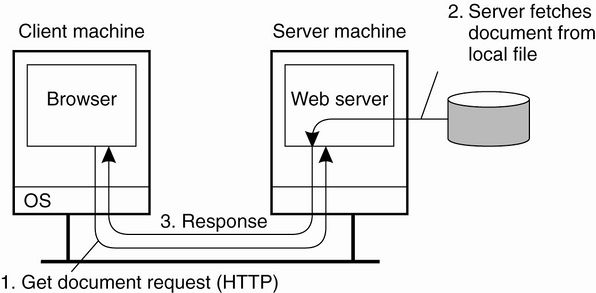
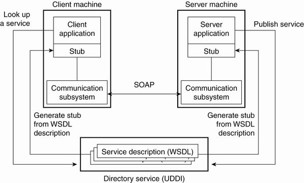
Traditional Web-Based Systems vs Web Services-Based Systems:

Traditional Web-Based Systems

Web services based systems

Creating - Deploying and Testing a Java Web Service using NetBeans

Esta sección fue realizada a partir de la siguiente presentación, la cual forma parte del material del curso de Big Data del Prof. Muhammad Iqbal: File:Lecture_4-Big_Data_integration-Web_Service.pptx

El proyecto NetBeans que contiene el Java Web Service resultante de este tutorial: File:CalculatorWSApplication.zip

Netbeans 6.5 - 9 and Java EE enable programmers to "publish (deploy)" and/or "consume (client request)" web services In Netbeans, you focus on the logic of the web service and let the IDE handle the web service's infrastructure.

• We first need to to do some configuration in NetBeans:
  • Go to /usr/local/netbeans-8.2/etc/netbeans.conf:
    • Find the line: netbeans_default_options
    • If -J-Djavax.xml.accessExternalSchema=all is not between the quotes then paste it in.

• If you are deploying to the GlassFish Server you need to modify the configuration file of the GlassFish Server (domain.xml):
  • /usr/local/glassfish-4.1.1/glassfish/domains/domain1/config/domain.xml
    • Find : <java-config
    • Check the jvm-options for the following configuration: <jvm-options>-Djavax.xml.accessExternalSchema=all</jvm-options>
    • It should be there by default, if not paste it in, save file and exit
    • You can now start Netbeans IDE

• Create a Web Service in NetBeans- Locally
  • Choose File > New Project:
  • Select Web Application from the Java Web category
  • Change Project Name: to CalculatorWSApplication
  • Set the server to GlassFish 4.1.1
  • Set Java EE Version: Java EE 7 Web
  • Set Context path: /CalculatorWSApplication
  • After that you should now have a project created in the Projects view on the left hand side.

• Creating a WS from a Java Class:

• Right-click the CalculatorWSApplication node and choose New > Web Service.

• If the option is not there choose Other > Web Services > Web Service

• Click Next
• Name the web service CalculatorWS and type com.hduser.calculator in Package. Leave Create Web Service from Scratch selected.
• Select Implement Web Service as a Stateless Session Bean.
• Click Finish. The Projects window displays the structure of the new web service and the Java class (CalculatorWS.java) is generate and automatically shown in the editor area. A default hello web service is created by Netbeans.

• Adding an Operation to the WS (CalculatorWS.java):

• Open CalculatorWS.java WS.
• Change to the Design view in the editor.
• Click the Add operation button.
• In the upper part of the Add Operation dialog box, type add in Name and type int' in the Return Type drop-down list.
• In the lower part of the Add Operation dialog box, click Add and create a parameter of type int named num_1.
• Click Add again and create a parameter of type int called num_2.
• Click OK at the bottom of the panel to add the operation.
• Remove the default hello operation: Right click on hello operation and choose: Remove Operation
• Click on the source view to go back to view the code in the editor.
• You will see the default hello code is gone and the new add method is now there instead.
• Now we have to alter the code to look like this.

package com.adelo.calculator;

import javax.jws.WebService;
import javax.jws.WebMethod;
import javax.jws.WebParam;
import javax.ejb.Stateless;

@WebService(serviceName = "CalculatorWS")
@Stateless()
public class CalculatorWS {

    /**
     * Web service operation
     */
    @WebMethod(operationName = "add")
    public int add(@WebParam(name = "num_1") int num_1, @WebParam(name = "num_2") int num_2) {
        //TODO write your implementation code here:
        int result = num_1 + num_2;
        return result;
    }
}

• Well done, you have just created your first Web Service.

• To test the Web service drop down the Web Services directory and right click on CalculatorWSApplication.
• Choose Test Web service.
• Netbeans throws an error: It is letting us know that we have not deployed our Web Service.

• Right click on the main Project node and select deploy

• Testing the WS:

• Deploying the Web Service will automatically start the GlassFish server. Allow the server to start, this will take a little while. You can check the progress by clicking on the GlassFish tab at the bottom of the IDE.
• Wait until you see: «CalculatorWSApplication was successfully deployed in 9,912 milliseconds»
• Now you can right click on the Web Service as before and choose Test Web Service.
• The browser will open and you can now test the Web service and view the WSDL file.
• You can also view the Soap Request and Response.

Understanding a Web Service Java Class

• Each new web service class created with the JAX-WS APIs is a POJO (plain old Java object)

• You do not need to extend a class or implement an interface to create a Web service.

• When you compile a class that uses the following JAX-WS 2.0 annotations, the compiler creates the compiled code framework that allows the web service to wait for and respond to client requests:

• @WebService(«Optional elements»)

• Indicates that a class represents a web service.
• Optional element name specifies the name of the proxy class that will be generated for the client.
• Optional element serviceName specifies the name of the class that the client uses to obtain a proxy object.
• Netbeans places the @WebService annotation at the beginning of each new web service class you create.
• You can add the optional name and serviceName this way: @WebService(serviceName = "CalculatorWS")

• @WebMethod(«Optional elements»)

• Methods that are tagged with the @WebMethod annotation can be called remotely.
• Methods that are not tagged with @WebMethod are not accessible to clients that consume the web service.
• Optional operationName element to specify the method name that is exposed to the web service's client.

• @WebParam annotation(«Optional elements»)

• Optional element name indicates the parameter name that is exposed to the web service's clients.

Consuming the Web Service

Netbeans 6.5 - 9 and Java EE enable programmers to "publish (deploy)" and/or "consume (client request)" web services

Creating a Java Web Application that consumes a Web Service

El proyecto NetBeans resultante de esta sección: File:CalculatorWSJSPClient.zip

• Now that we have a web service we need a client to consume it.
• Choose File > New Project
• Select Web Application from the Java Web category
• Name the project CalculatorWSJSPClient
• Leave the server and java version as before and click Finish.

• Expand the Web Pages node under the project node and delete index.html.
• Right-click the Web Pages node and choose New > JSP in the popup menu.
  • If JSP is not available in the popup menu, choose New > Other and select JSP in the Web category of the New File wizard.
• Type index for the name of the JSP file in the New File wizard. Click Finish to create the JSP (Java Server Page)

• Right-click the CalculatorWSJSPClient node and choose New > Web Service Client.
  • If the option is not there choose Other > Web Services > Web Service Client

• To consume a locally Java Web Service:
  • Select Project as the WSDL source. Click Browse. Browse to the CalculatorWS web service in the CalculatorWSApplication project. When you have selected the web service, click OK.

• To consume a Web Service in another location: For example, the one that is available at http://vhost3.cs.rit.edu/SortServ/Service.svc?singleWsdl
  • Specify the WSDL URL as: http://vhost3.cs.rit.edu/SortServ/Service.svc?singleWsdl
  • (we are going to explain more about this WS in the next section. For this tutorial we are going to continue with the example of our locally Java Web Service CalculatorWS).

• Do not select a package name. Leave this field empty.
• Leave the other settings as default and click Finish.

• The WSDL gets parsed and generates the .java
• The Web Service References directory now contains the add method we created in our web service.
• Drag and drop the add method just below the H1 tags in index.jsp
• The Code will be automatically generated.
• Change the values of num_1 and num_2 to any two numbers e.g. 5 and 5 as per test earlier.
• Remove the TODO line from the catch block of the code and paste in:

out.println("exception" + ex);

If there is an error this will help us identify the problem.

• IMPORTANT Once you close Netbeans you are shutting down your server. If you want to reuse a Web Service you must re-deploy.

Creating a Java project that consumes a Web Service

Esta sección fue realizada a partir del siguiente tutorial: File:Creating_a_Java_project_that_consumes_a_Web_Service.zip

El proyecto NetBeans resultante de esta sección: File:SortClient.zip

This document provides step-by-step instructions to consume a web service in Java using NetBeans IDE.

In the project, we will invoke a sorting web service through its WSDL link: http://vhost3.cs.rit.edu/SortServ/Service.svc?singleWsdl

• Step 1 - Createa JavaProject:
  • We are going to name it: SortClient

• Step 2 - Generate a Web Service Client:
  • After the Java Project has been created, go to the Project Tree Structure, Right click on Project and select New and then choose Web Service Client.
  • Specify the WSDL URL as: http://vhost3.cs.rit.edu/SortServ/Service.svc?singleWsdl
  • Click Finish

• Step 3 - Invoke the Service:
  • Expand the Web Service References until you see the operation lists. Drag the operation you want to invoke to the source code window, such as "GetKey". A piece of code is automatically generated to invoke that operation.
  • Drag MergeSort to the source code window and the corresponding code is automatically generated,too.
  • In the main function, add the code to call the two functions: getKey() and mergeSort();As it is a call to a remote service, RemoteException needs to be listed in the throws cause

Another example 1 - Creating a Java Web Application that consume a Web Service using NetBeans

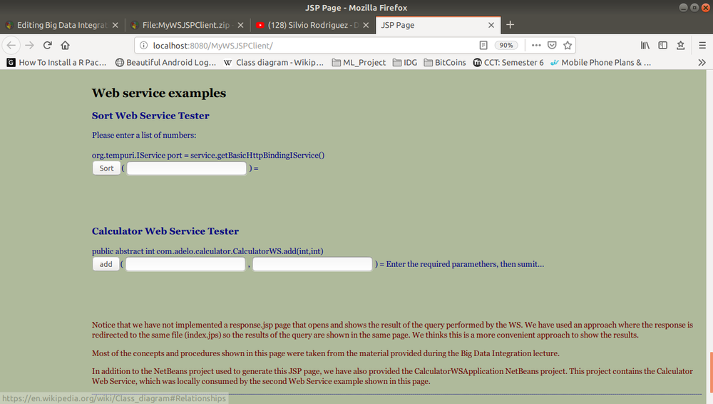
This is the assignment I did for this part of the course, the Netbeans project is available here: File:MyWSJSPClient.zip

The following image is the Web Application created from MyWSJSPClient:

Java Web Application that consume two Web Services. The Sort Web Service Tester is consume from http://vhost3.cs.rit.edu/SortServ/Service.svc?Wsdl. The Calculator Web Service is locally consumed from the CalculatorWSApplication project we created at Big Data Integration#Creating - Deploying and Testing a Java Web Service using NetBeans

Another example 2 - Creating a Java Web Application that consume a Web Service using NetBeans

In this page we can find another example of a Java EE web application that contains a web service: https://netbeans.org/kb/docs/websvc/flower_overview.html

Data analysis

Data analysis is the process of inspecting, cleansing, transforming, and modelling data with a goal of discovering useful information, suggesting conclusions, and supporting decision-making.

Data mining is a particular data analysis technique that focuses on the modelling and knowledge discovery for predictive rather than purely descriptive purposes, while business intelligence covers data analysis that relies heavily on aggregation, focusing on business information.

In statistical applications, data analysis can be divided into:

• Descriptive statistics,
• Exploratory data analysis (EDA), and
• Confirmatory data analysis (CDA).

In particular, data analysis typically includes data retrieval and data cleaning (pre-processing) stages.

Exploratory Data: In statistics, the exploratory data analysis (EDA) is an approach to analyzing data sets to summarize their main characteristics, often with visual methods.

Confirmatory Analysis: In statistics, confirmatory analysis (CA) or confirmatory factor analysis (CFA) is a special form of factor analysis, most commonly used in social research.

Empirical Research:

Statistical Significance:

Descriptive Data Analysis:

• Rather than find hidden information in the data, descriptive data analysis looks to summarise the dataset.
• They are commonly implemented measures included in the descriptive data analysis:
  • Central tendency (mean, mode, median)
  • Variability (standard deviation, min/max)

Exploratory Data Analysis:

• Generate Summaries and make general statements about the data, and its relationships within the data is the heart of Exploratory Data Analysis.

• We generally make assumptions on the entire population but mostly just work with small samples. Why are we allowed to do this??? Two important definitions:
  • Population: A precise definition of all possible outcomes, measurements or values for which inference will be made about.
  • Sample: A portion of the population which is representative of the population (at least ideally).

Types of Variable: https://statistics.laerd.com/statistical-guides/types-of-variable.php

Central tendency

https://statistics.laerd.com/statistical-guides/measures-central-tendency-mean-mode-median.php

A central tendency (or measure of central tendency) is a single value that attempts to describe a set of data by identifying the central position within that set of data.

The mean (often called the average) is most likely the measure of central tendency that you are most familiar with, but there are others, such as the median and the mode.

The mean, median and mode are all valid measures of central tendency, but under different conditions, some measures of central tendency become more appropriate to use than others. In the following sections, we will look at the mean, mode and median, and learn how to calculate them and under what conditions they are most appropriate to be used.

Mean

Mean (Arithmetic)

The mean (or average) is the most popular and well known measure of central tendency.

The mean is equal to the sum of all the values in the data set divided by the number of values in the data set.

So, if we have $n$ values in a data set and they have values $x_{1},x_{2},...,x_{n},$the sample mean, usually denoted by ${\bar {x}}$ (pronounced x bar), is:

${\bar {x}}={\frac {(x_{1}+x_{2}+...+x_{n})}{n}}={\frac {\sum x}{n}}$

The mean is essentially a model of your data set. It is the value that is most common. You will notice, however, that the mean is not often one of the actual values that you have observed in your data set. However, one of its important properties is that it minimises error in the prediction of any one value in your data set. That is, it is the value that produces the lowest amount of error from all other values in the data set.

An important property of the mean is that it includes every value in your data set as part of the calculation. In addition, the mean is the only measure of central tendency where the sum of the deviations of each value from the mean is always zero.

When not to use the mean

The mean has one main disadvantage: it is particularly susceptible to the influence of outliers. These are values that are unusual compared to the rest of the data set by being especially small or large in numerical value. For example, consider the wages of staff at a factory below:

Staff	1	2	3	4	5	6	7	8	9	10
Salary	$15k$	$18k$	$16k$	$14k$	$15k$	$15k$	$12k$	$17k$	$90k$	$95k$

The mean salary for these ten staff is $30.7k. However, inspecting the raw data suggests that this mean value might not be the best way to accurately reflect the typical salary of a worker, as most workers have salaries in the $12k to 18k range. The mean is being skewed by the two large salaries. Therefore, in this situation, we would like to have a better measure of central tendency. As we will find out later, taking the median would be a better measure of central tendency in this situation.

Another time when we usually prefer the median over the mean (or mode) is when our data is skewed (i.e., the frequency distribution for our data is skewed). If we consider the normal distribution - as this is the most frequently assessed in statistics - when the data is perfectly normal, the mean, median and mode are identical. Moreover, they all represent the most typical value in the data set. However, as the data becomes skewed the mean loses its ability to provide the best central location for the data because the skewed data is dragging it away from the typical value. However, the median best retains this position and is not as strongly influenced by the skewed values. This is explained in more detail in the skewed distribution section later in this guide.

Mean in R

mean(iris$Sepal.Width)

Median

The median is the middle score for a set of data that has been arranged in order of magnitude. The median is less affected by outliers and skewed data. In order to calculate the median, suppose we have the data below:

65	55	89	56	35	14	56	55	87	45	92

We first need to rearrange that data into order of magnitude (smallest first):

14	35	45	55	55	56	56	65	87	89	92

Our median mark is the middle mark - in this case, 56. It is the middle mark because there are 5 scores before it and 5 scores after it. This works fine when you have an odd number of scores, but what happens when you have an even number of scores? What if you had only 10 scores? Well, you simply have to take the middle two scores and average the result. So, if we look at the example below:

65	55	89	56	35	14	56	55	87	45

We again rearrange that data into order of magnitude (smallest first):

14	35	45	55	55	56	56	65	87	89

Only now we have to take the 5th and 6th score in our data set and average them to get a median of 55.5.

Median in R

median(iris$Sepal.Length)

Mode

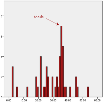
The mode is the most frequent score in our data set. On a histogram it represents the highest bar in a bar chart or histogram. You can, therefore, sometimes consider the mode as being the most popular option. An example of a mode is presented below:

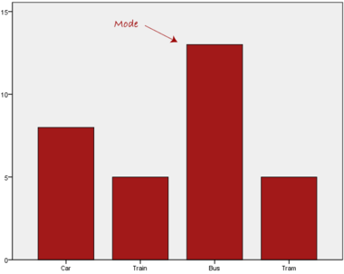
Normally, the mode is used for categorical data where we wish to know which is the most common category, as illustrated below:

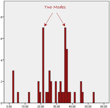
We can see above that the most common form of transport, in this particular data set, is the bus. However, one of the problems with the mode is that it is not unique, so it leaves us with problems when we have two or more values that share the highest frequency, such as below:

We are now stuck as to which mode best describes the central tendency of the data. This is particularly problematic when we have continuous data because we are more likely not to have any one value that is more frequent than the other. For example, consider measuring 30 peoples' weight (to the nearest 0.1 kg). How likely is it that we will find two or more people with exactly the same weight (e.g., 67.4 kg)? The answer, is probably very unlikely - many people might be close, but with such a small sample (30 people) and a large range of possible weights, you are unlikely to find two people with exactly the same weight; that is, to the nearest 0.1 kg. This is why the mode is very rarely used with continuous data.

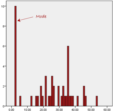
Another problem with the mode is that it will not provide us with a very good measure of central tendency when the most common mark is far away from the rest of the data in the data set, as depicted in the diagram below:

In the above diagram the mode has a value of 2. We can clearly see, however, that the mode is not representative of the data, which is mostly concentrated around the 20 to 30 value range. To use the mode to describe the central tendency of this data set would be misleading.

To get the Mode in R

install.packages("modeest")
library(modeest)

> mfv(iris$Sepal.Width, method = "mfv")

Skewed Distributions and the Mean and Median

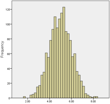
We often test whether our data is normally distributed because this is a common assumption underlying many statistical tests. An example of a normally distributed set of data is presented below:

When you have a normally distributed sample you can legitimately use both the mean or the median as your measure of central tendency. In fact, in any symmetrical distribution the mean, median and mode are equal. However, in this situation, the mean is widely preferred as the best measure of central tendency because it is the measure that includes all the values in the data set for its calculation, and any change in any of the scores will affect the value of the mean. This is not the case with the median or mode.

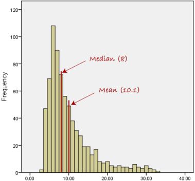
However, when our data is skewed, for example, as with the right-skewed data set below:

we find that the mean is being dragged in the direct of the skew. In these situations, the median is generally considered to be the best representative of the central location of the data. The more skewed the distribution, the greater the difference between the median and mean, and the greater emphasis should be placed on using the median as opposed to the mean. A classic example of the above right-skewed distribution is income (salary), where higher-earners provide a false representation of the typical income if expressed as a mean and not a median.

If dealing with a normal distribution, and tests of normality show that the data is non-normal, it is customary to use the median instead of the mean. However, this is more a rule of thumb than a strict guideline. Sometimes, researchers wish to report the mean of a skewed distribution if the median and mean are not appreciably different (a subjective assessment), and if it allows easier comparisons to previous research to be made.

Summary of when to use the mean, median and mode

Please use the following summary table to know what the best measure of central tendency is with respect to the different types of variable:

Type of Variable	Best measure of central tendency
Nominal	Mode
Ordinal	Median
Interval/Ratio (not skewed)	Mean
Interval/Ratio (skewed)	Median

For answers to frequently asked questions about measures of central tendency, please go to: https://statistics.laerd.com/statistical-guides/measures-central-tendency-mean-mode-median-faqs.php

Measures of Variation

Range

The Range just simply shows the min and max value of a variable.

In R:

> min(iris$Sepal.Width)
> max(iris$Sepal.Width)
> range(iris$Sepal.Width)

Range can be used on Ordinal, Ratio and Interval scales

Quartile

https://statistics.laerd.com/statistical-guides/measures-of-spread-range-quartiles.php

Quartiles tell us about the spread of a data set by breaking the data set into quarters, just like the median breaks it in half.

For example, consider the marks of the 100 students, which have been ordered from the lowest to the highest scores.

• The first quartile (Q1): Lies between the 25th and 26th student's marks.
  • So, if the 25th and 26th student's marks are 45 and 45, respectively:
    • (Q1) = (45 + 45) ÷ 2 = 45
• The second quartile (Q2): Lies between the 50th and 51st student's marks.
  • If the 50th and 51th student's marks are 58 and 59, respectively:
    • (Q2) = (58 + 59) ÷ 2 = 58.5
• The third quartile (Q3): Lies between the 75th and 76th student's marks.
  • If the 75th and 76th student's marks are 71 and 71, respectively:
    • (Q3) = (71 + 71) ÷ 2 = 71

In the above example, we have an even number of scores (100 students, rather than an odd number, such as 99 students). This means that when we calculate the quartiles, we take the sum of the two scores around each quartile and then half them (hence Q1= (45 + 45) ÷ 2 = 45) . However, if we had an odd number of scores (say, 99 students), we would only need to take one score for each quartile (that is, the 25th, 50th and 75th scores). You should recognize that the second quartile is also the median.

Quartiles are a useful measure of spread because they are much less affected by outliers or a skewed data set than the equivalent measures of mean and standard deviation. For this reason, quartiles are often reported along with the median as the best choice of measure of spread and central tendency, respectively, when dealing with skewed and/or data with outliers. A common way of expressing quartiles is as an interquartile range. The interquartile range describes the difference between the third quartile (Q3) and the first quartile (Q1), telling us about the range of the middle half of the scores in the distribution. Hence, for our 100 students:

$Interquartile\ range=Q3-Q1=71-45=26$

However, it should be noted that in journals and other publications you will usually see the interquartile range reported as 45 to 71, rather than the calculated $Interquartile\ range.$

A slight variation on this is the $semi{\text{-}}interquartilerange,$which is half the $Interquartile\ range.$Hence, for our 100 students:

$Semi{\text{-}}Interquartile\ range={\frac {Q3-Q1}{2}}={\frac {71-45}{2}}=13$

Quartile in R

quantile(iris$Sepal.Length)

Result 
0%    25%    50%    75%    100% 
4.3   5.1    5.8    6.4    7.9

0% and 100% are equivalent to min max values.

Box Plots

boxplot(iris$Sepal.Length,
       col = "blue", 
       main="iris dataset", 
       ylab = "Sepal Length")

Variance

https://statistics.laerd.com/statistical-guides/measures-of-spread-absolute-deviation-variance.php

Another method for calculating the deviation of a group of scores from the mean, such as the 100 students we used earlier, is to use the variance. Unlike the absolute deviation, which uses the absolute value of the deviation in order to "rid itself" of the negative values, the variance achieves positive values by squaring each of the deviations instead. Adding up these squared deviations gives us the sum of squares, which we can then divide by the total number of scores in our group of data (in other words, 100 because there are 100 students) to find the variance (see below). Therefore, for our 100 students, the variance is 211.89, as shown below:

$variance=\sigma ={\frac {\sum (X-\mu )^{2}}{N}}$

$\mu :{\text{Mean}};\ \ \ X:{\text{Score}};\ \ \ N:{\text{Number of scores}}$

• Variance describes the spread of the data.
• It is a measure of deviation of a variable from the arithmetic mean.
• The technical definition is the average of the squared differences from the mean.
• A value of zero means that there is no variability; All the numbers in the data set are the same.
• A higher number would indicate a large variety of numbers.
  

Variance in R

var(iris$Sepal.Length)

Standard Deviation

https://statistics.laerd.com/statistical-guides/measures-of-spread-standard-deviation.php

The standard deviation is a measure of the spread of scores within a set of data. Usually, we are interested in the standard deviation of a population. However, as we are often presented with data from a sample only, we can estimate the population standard deviation from a sample standard deviation. These two standard deviations - sample and population standard deviations - are calculated differently. In statistics, we are usually presented with having to calculate sample standard deviations, and so this is what this article will focus on, although the formula for a population standard deviation will also be shown.

The sample standard deviation formula is:

$s={\sqrt {\frac {\sum (X-{\bar {X}})^{2}}{n-1}}}$

${\bar {X}}:{\text{Sample mean}};\ \ \ n:{\text{Number of scores in the sample}}$

The population standard deviation formula is:

$\sigma ={\sqrt {\frac {\sum (X-\mu )^{2}}{n}}}$

$\mu :{\text{population mean}}$

• The Standard Deviation is the square root of the variance.
• This measure is the most widely used to express deviation from the mean in a variable.
• The higher the value the more widely distributed are the variable data values around the mean.
• Assuming the frequency distributions approximately normal, about 68% of all observations are within +/- 1 standard deviation.
• Approximately 95% of all observations fall within two standard deviations of the mean (if data is normally distributed).

Standard Deviation in R

sd(iris$Sepal.Length)

Z Score

• z-score represents how far from the mean a particular value is based on the number of standard deviations.
• z-scores are also known as standardized residuals
• Note: mean and standard deviation are sensitive to outliers

> x <-((iris$Sepal.Width) - mean(iris$Sepal.Width))/sd(iris$Sepal.Width)
> x 
> x[77] #choose a single row # or this
> x <-((iris$Sepal.Width[77]) - mean(iris$Sepal.Width))/sd(iris$Sepal.Width)
> x

Shape of Distribution

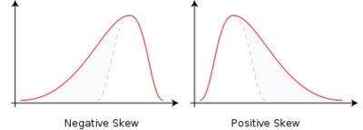
Skewness

• Skewness is a method for quantifying the lack of symmetry in the distribution of a variable.

• Skewness value of zero indicates that the variable is distributed symmetrically. Positive number indicate asymmetry to the left, negative number indicates asymmetry to the right.

Skewness in R

> install.packages("moments") and library(moments)
> skewness(iris$Sepal.Width)

Histograms in R

> hist(iris$Petal.Width)

Kurtosis

• Kurtosis is a measure that gives indication in terms of the peak of the distribution.

• Variables with a pronounced peak toward the mean have a high Kurtosis score and variables with a flat peak have a low Kurtosis score.

Kurtosis in R

> kurtosis(iris$Sepal.Length)

Correlations

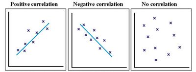
Correlation give us a measure of the relation between two or more variables.

• Positive correlation: The points lie close to a straight line, which has a positive gradient. This shows that as one variable increases the other increases.

• Negative correlation: The points lie close to a straight line, which has a negative gradient. This shows that as one variable increases the other decreases.

• No correlation: There is no pattern to the points. This shows that there is no correlation between the tow variables.

Simple Linear Correlation

• Looking for the extent to which two values of the two variables are proportional to each other.

• Summarised by a straight line.

• This line is called a Regression Line or a Least Squares Line.

• It is determined by maintaining the lowest possible sum of squared distances between the data points and the line.

• We must use interval scales or ratio scales for this type of analysis.

Simple Linear Correlation in R

Example 1:

> install.packages('ggplot2')
> library(ggplot2)
> data("iris")

> ggplot(iris, aes(x=Sepal.Length, y=Sepal.Width)) + 
         geom_point(color='black') + 
         geom_smooth(method=lm, se=FALSE, fullrange=TRUE)

Example 2:

> library(ggplot2)
> data("iris")
> ggplot(iris, aes(x=Petal.Length, y=Sepal.Length)) + 
         geom_point(color='black') + 
         geom_smooth(method=lm, se=FALSE, fullrange=TRUE)