Difference between revisions of "Data Science"

Irish Government Data Portal	https://data.gov.ie/
UK Government Data Portal	https://data.gov.uk/
UK National Health Service Data	https://digital.nhs.uk/data-and-information
EU Open Data Portal	http://data.europa.eu/euodp/en/data/
US Government Data Portal	https://www.data.gov/
Canadian Government Data Portal	https://open.canada.ca/en/open-data
Indian Government Open Data	https://data.gov.in/
World Bank	https://data.worldbank.org/
International Monetary Fund	https://www.imf.org/en/Data
World Health Organisation	http://www.who.int/gho/en/
UNICEF	https://data.unicef.org/
Federal Drug Administration	https://www.fda.gov/Drugs/InformationOnDrugs/ucm079750.htm
Google Public Data Explorer	https://www.google.com/publicdata/directory
Human Rights Data Analysis Group	https://hrdag.org/
Armed Conflict Data	http://www.pcr.uu.se/research/UCDP/
Amazon Web Services Open Data Registry	https://registry.opendata.aws/
Pew Research Datasets	http://www.pewinternet.org/datasets/
CERN Open Data	http://opendata.cern.ch/
Kaggle	https://www.kaggle.com/
UCI Machine Learning Repository	https://archive.ics.uci.edu/ml/index.php
Open Data Network	https://www.opendatanetwork.com/
Linked Open Data - University of Münster	https://www.uni-muenster.de/LODUM/
US National Climate Data	https://www.ncdc.noaa.gov/data-access/quick-links#loc-clim
US Medicare Hospital Quality Data	https://data.medicare.gov/data/hospital-compare
Yelp Data	https://www.yelp.com/dataset/challenge
US Census Data	https://www.census.gov/data.html
Broad Institute Cancer Program Data	http://portals.broadinstitute.org/cgi-bin/cancer/datasets.cgi
National Centers for Environmental Information	https://www.ncdc.noaa.gov/data-access
Centers for Disease Control and Prevention	https://www.cdc.gov/datastatistics/
Open Data Monitor	https://opendatamonitor.eu/
Plenario	http://plenar.io/
British Film Institute	http://www.bfi.org.uk/education-research/film-industry-statistics-research
Edinburgh University Datasets	http://www.inf.ed.ac.uk/teaching/courses/dme/html/datasets0405.html
DataHub	http://datahub.io

What is data

It is difficult to define such a broad concept, but the definition that I like it that data is a collection (or any set) of characters such as numbers, words, images, files, that represent measurements, observations, or just descriptions, that are gathered for some purpose. https://www.mathsisfun.com/data/data.html https://www.computerhope.com/jargon/d/data.htm

Qualitative vs quantitative data

https://learn.g2.com/qualitative-vs-quantitative-data

Taken from https://www.mathsisfun.com/data/data.html

Qualitative data is descriptive information (it describes something)
Quantitative data is numerical information (numbers)

In short, we can say that the difference is that Quantitative data can be counted, measured, and expressed using numbers. Qualitative data is descriptive and conceptual. Qualitative data can be categorized based on traits and characteristics.

Quantitative data is objective, to-the-point, and conclusive, while qualitative data is subjective, interpretive, and exploratory.

Qualitative data is descriptive information (it describes something)

Qualitative data is non-statistical and is typically unstructured or semi-structured in nature. This data isn’t necessarily measured using hard numbers used to develop graphs and charts. Instead, it is categorized based on properties, attributes, labels, and other identifiers.

Qualitative data can be generated through:

Texts and documents
Audio and video recordings
Images and symbols
Interview transcripts and focus groups
Observations and notes

Quantitative data is numerical information (numbers)

Contrary to qualitative data, quantitative data is statistical and is typically structured in nature – meaning it is more rigid and defined. This type of data is measured using numbers and values

Quantitative data can be generated through:

Tests
Experiments
Surveys
Market reports
Metrics

Discrete and continuous data

Taken from https://www.youtube.com/watch?v=cz4nPSA9rlc

https://www.youtube.com/watch?v=cz4nPSA9rlc

Quantitative data can be discrete or continuous.

Continuous data ca take on any value in an interval.

We usually say that continuous data is measured.
Ex1. Temperature: $83.6$ ºF, $99.46$ ºF. Temperature can be any value between an interval and it is measured (no counted)
Ex2.

Discrete data can only have specific values.

We usually say that discrete data is counted.
Discrete data are usually (but not always) whole numbers $[-2,-1,0,1,2,3,4,5...]$
Ex. Possible values on a dice $[1,2,3,4,5,6]$
Ex2. Shoe size of $[3.5,4,4.5,5...]$ . They are not whole numbers but can not be any number.

Structured vs Unstructured data

https://learn.g2.com/structured-vs-unstructured-data

http://troindia.in/journal/ijcesr/vol3iss3/36-40.pdf

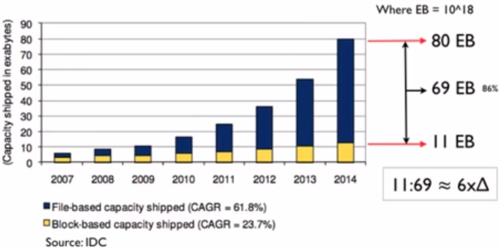
It is important to highlight that the huge increase in data in the last 10 years has been driven by the increase in unstructured data. Currently, some estimations indicate that there are around 300 exabytes of data, of which around 80% is unstructured data.

The prefix exa indicates multiplication by the sixth power of 1000 ( $10^{18}$ ). $1EB=10^{18}bytes=1000^{6}bytes=1,000,000,000,000,000,000B$

Some estimates also indicate that the amount of data is doubling every 2 years.

Source: IDC. Taken from https://www.youtube.com/watch?v=WBU7sW1jy2o
Taken from http://mis587pushkarmaid.blogspot.com/2016/03/big-unstructured-data-vs-structured.html

Source: Taken from https://docplayer.net/3430405-Self-service-bi-for-big-data-applications-using-apache-drill.html
Taken from https://itbrandpulse.com/enterprise-storage-tco-case-study/

Structured data

Structured data is organized within fixed fields or columns, usually in relational databases (or spreadsheets) so it can be easily queried with SQL. https://learn.g2.com/structured-vs-unstructured-data https://www.talend.com/resources/structured-vs-unstructured-data/

An example of Structured data is all the data that is usually associated with the ERP, such as «Customer data (CRM)» «Human resource data», «Accounting data»

the typical company's database where the company stores, for example, «Employees», «Projects» and «Equipment» data:

«Employees»: f_name, s_name, dob, address

Unstructured data

It doesn't fit easily into a spreadsheet or a relational database.

Examples of unstructured data include: https://www.m-files.com/blog/what-is-structured-data-vs-unstructured-data/

Media: Audio and video files, images
Text files: Word docs, PowerPoint presentations, email, chat logs
Email: There’s some internal metadata structure, so it’s sometimes called semi-structured, but the message field is unstructured and difficult to analyze with traditional tools.
Social Media: Data from social networking sites like Facebook, Twitter, and LinkedIn
Mobile data: Text messages, locations
Communications: Chat, call recordings
Those examples are largely human-generated, but machine-generated data can also be unstructured: satellite images, scientific data, surveillance images, and video, weather sensor data.

Semi-structured data

The line between Semi-structured data and Unstructured data has always been unclear. Semi-structured data is usually referred to as information that is not structured in a traditional database but contains some organizational properties that make its processing easier. For example, NoSQL documents are considered to be semi-structured data since they contain keywords that can be used to process the documents easier. https://www.youtube.com/watch?v=dK4aGzeBPkk

Data Levels and Measurement

Levels of Measurement - Measurement scales

https://www.statisticssolutions.com/data-levels-and-measurement/

There are four Levels of Measurement in research and statistics: Nominal, Ordinal, Interval, and Ratio.


Nominal	A nominal variable is one in which values serve only as labels. Nominal values don't have any meaningful order or carry any mathematical meaning. Nominal data cannot be used to perform many statistical computations, such as mean and standard deviation. Even if the values are numbers. For example, if we want to categorize males and females, we could use a number of 1 for male, and 2 for female. However, the values of 1 and 2 in this case don't have any meaningful order or carry any mathematical meaning. They are simply used as labels. https://www.statisticssolutions.com/data-levels-and-measurement/ Nominal values serve only as labels. Nominal values don't have any meaningful order or carry any mathematical meaning Nominal data cannot be used to perform many statistical computations, such as mean and standard deviation Another examples: For an attribute "outlook" from weather data, potential values could be "sunny", "overcast", and "rainy".
Ordinal	Values of ordinal variables have a meaningful order. However, no distance between values is defined. Therefore, only comparison operators make sense. Mathematical operations such as addition, multiplication, etc. do not make sense. For example, an education level attribute (with possible values of high school, undergraduate degree, and graduate degree) would be an ordinal variable. There is a definitive order to the categories (i.e., graduate is higher than undergraduate, and undergraduate is higher than high school), but we cannot make any other arithmetic assumption. For instance, we cannot assume that the difference in education level between undergraduate and high school is the same as the difference between graduate and undergraduate. Values have a meaningful order However, no distance between values is defined Only comparison operators make sense. Mathematical operations such as addition, multiplication, etc. do not. We can use frequencies, percentages, and certain non-parametric statistics with ordinal data. However, means, standard deviations, and parametric statistical tests are generally not appropriate to use with ordinal data. https://www.statisticssolutions.com/data-levels-and-measurement/ Distinction between nominal and ordinal not always clear (e.g., attribute “outlook”) Another examples: For the attribute “temperature” in weather data potential values could be: "hot" > "warm" > "cool"
Interval	For interval variables, we can make arithmetic assumptions about the degree of difference between values. An example of an interval variable would be temperature. We can correctly assume that the difference between 70 and 80 degrees is the same as the difference between 80 and 90 degrees. However, the mathematical operations of multiplication and division do not apply to interval variables. For instance, we cannot accurately say that 100 degrees is twice as hot as 50 degrees. Additionally, interval variables often do not have a meaningful zero-point. For example, a temperature of zero degrees (on Celsius and Fahrenheit scales) does not mean a complete absence of heat. An interval variable can be used to compute commonly used statistical measures such as the average (mean), standard deviation, and the Pearson correlation coefficient. https://www.statisticssolutions.com/data-levels-and-measurement/
Ratio	All arithmetic operations are possible on a ratio variable. An example of a ratio variable would be weight (e.g., in pounds). We can accurately say that 20 pounds is twice as heavy as 10 pounds. Additionally, ratio variables have a meaningful zero-point (e.g., exactly 0 pounds means the object has no weight). Other examples of ratio variables include gross sales of a company, the expenditure of a company, the income of a company, etc. A ratio variable can be used as a dependent variable for most parametric statistical tests such as t-tests, F-tests, correlation, and regression. https://www.statisticssolutions.com/data-levels-and-measurement/


	Nominal	Ordinal	Interval	Ratio
The "order" of values is known		✔	✔	✔
"Counts", aka, "Frequency of Distribution"	✔	✔	✔	✔
Mode	✔	✔	✔	✔
Median		✔	✔	✔
Mean			✔	✔
Can quantify the difference between each value			✔	✔
Can add or subtract values			✔	✔
Can multiple and divide values				✔
Has "true zero"				✔

In Practice:

Most schemes accommodate just two levels of measurement: nominal and ordinal
Nominal attributes are also called "categorical", "enumerated", or "discrete". However, "enumerated" and "discrete" imply order
There is one special case: dichotomy (otherwise known as a "boolean" attribute)
Ordinal attributes are called "numeric", or "continuous", however "continuous" implies mathematical continuity

What is an example

Taken from https://www.youtube.com/watch?v=XAdTLtvrkFM

An example, also known in statistics as an observation, is an instance of the phenomenon that we are studying. An observation is characterized by a set of attributes.

Another definition: A recording of the qualities and quantities of an observable phenomenon in the natural world. An observation is characterized by a set of attributes. This could include what we can see, hear, feel, or measure with sensors. https://www.youtube.com/watch?v=XAdTLtvrkFM

In data science, we record observations on the rows of a table.

For example, imaging that we are recording the vital signs of a patient. For each observation we would record the «date of the observation», the «patient's heart» rate, and the «temperature»

What is a dataset

[Noel Cosgrave slides]

A dataset is typically a matrix of observations (in rows) and their attributes (in columns).

It is usually stored as:

Flat-file (comma-separated values (CSV)) (tab-separated values (TSV)). A flat file can be a plain text file or a binary file.
Database table
Spreadsheets

It is by far the most common form of data used in practical data mining and predictive analytics. However, it is a restrictive form of input as it is impossible to represent relationships between observations.

What is Metadata

Metadata is information about the data that encodes background knowledge. It can be thought of as "data about the data" and contains: [Noel Cosgrave slides]

Information about the data types for each variable in the data.
Description of the variable.
Restrictions on values the variable can hold.
Details of special orderings, such as circular orderings(e.g. degrees in compass, time of day)

What is Data Science

What is Data Science - Data Analysis - Data Analytics - Predictive Data Analytics - Data Mining - Machine Learning - Big Data - AI

https://www.loginworks.com/blogs/top-10-small-differences-between-data-analyticsdata-analysis-and-data-mining/

https://www.quora.com/What-is-the-difference-between-Data-Analytics-Data-Analysis-Data-Mining-Data-Science-Machine-Learning-and-Big-Data-1

Data Science

Data Science is a discipline that uses aspects of statistics, computer science, applied mathematics, and visualization techniques to get new insights and new knowledge from a vast amount of data http://makemeanalyst.com/what-is-data-science/

Data analysis

Data analysis is the process of extracting, cleansing, transforming, modeling, and visualizing data with the goal of uncovering useful information that can help in deriving conclusion and usually in taking decisions [EDUCBA]

Data analysis is a broader term that includes other stages that are not usually related to Data Analytics or Data Mining https://www.loginworks.com/blogs/top-10-small-differences-between-data-analyticsdata-analysis-and-data-mining/

Define a Business objective
Data collection (Extracting the data)
Data Integration: Multiple data sources are combined. http://troindia.in/journal/ijcesr/vol3iss3/36-40.pdf
Data Transformation: The data is transformed or consolidated into forms which are appropriate or valid for mining by performing various aggregation operations. http://troindia.in/journal/ijcesr/vol3iss3/36-40.pdf
Optimisation: Making the results more precise or accurate over time.

Data Mining

The process of discovering patterns in large data sets using machine learning, statistics, and database systems https://www.loginworks.com/blogs/top-10-small-differences-between-data-analyticsdata-analysis-and-data-mining/

We can say that Data Mining is a Data Analysis subset that focuses on:

Discovering hidden patterns
Developing predictive models (ML algorithms, Correlation)

Common methods in data mining are:

Clustering: It is the task of finding groups of data that are similar (grouping data that are similar together).

For example, in a Library, We can use clustering to group similar books together, so customers that are interested in a particular kind of book can see other similar books
Recommender Systems: Recommender systems are designed to recommend new items based on a user's tastes. They sometimes use clustering algorithms to predict a user's preferences based on the preferences of other users in the user's cluster.

Correlation

Classification

Big Data

Big data is an evolving term that describes massive amounts of structured, semi-structured, and unstructured data that has the potential to be mined for information but is too large to be processed and analyzed using traditional data tools.

Machine Learning

Al tratar de encontrar una definición para Machine Learning me di cuanta de que muchos expertos coinciden en que no hay una definición standard para ML.

En este post se explica bien la definición de ML: https://machinelearningmastery.com/what-is-machine-learning/

Estos vídeos también son excelentes para entender what ML is:

https://www.youtube.com/watch?v=f_uwKZIAeM0

https://www.youtube.com/watch?v=ukzFI9rgwfU

https://www.youtube.com/watch?v=WXHM_i-fgGo

https://www.coursera.org/lecture/machine-learning/what-is-machine-learning-Ujm7v

Una de las definiciones más citadas es la definición de Tom Mitchell. This author provides in his book Machine Learning a definition in the opening line of the preface:

Tom Mitchell

The field of machine learning is concerned with the question of how to construct computer programs that automatically improve with experience.

So, in short we can say that ML is about write computer programs that improve themselves.

Tom Mitchell also provides a more complex and formal definition:

Tom Mitchell

A computer program is said to learn from experience E with respect to some class of tasks T and performance measure P, if its performance at tasks in T, as measured by P, improves with experience E.

Don't let the definition of terms scare you off, this is a very useful formalism. It could be used as a design tool to help us think clearly about:

E: What data to collect.

T: What decisions the software needs to make.

P: How we will evaluate its results.

Suppose your email program watches which emails you do or do not mark as spam, and based on that learns how to better filter spam. In this case: https://www.coursera.org/lecture/machine-learning/what-is-machine-learning-Ujm7v

E: Watching you label emails as spam or not spam.

T: Classifying emails as spam or not spam.

P: The number (or fraction) of emails correctly classified as spam/not spam.

Styles of Learning - Types of Machine Learning

Supervised Learning

https://en.wikipedia.org/wiki/Supervised_learning

Supervised learning is the machine learning task of learning a function that maps an input to an output based on example input-output pairs.

In other words, It infers a function from labeled training data consisting of a set of training examples.

In supervised learning, each example is a pair consisting of an input object (typically a vector) and a desired output value (also called the supervisory signal).

A supervised learning algorithm analyzes the training data and produces an inferred function, which can be used for mapping new examples.

https://machinelearningmastery.com/supervised-and-unsupervised-machine-learning-algorithms/

The majority of practical machine learning uses supervised learning.

Supervised learning is when you have input variables (x) and an output variable (Y) and you use an algorithm to learn the mapping function from the input to the output.

$y=f(x)$

The goal is to approximate the mapping function so well that when you have new input data ( $x$ ) that you can predict the output variables ( $y$ ) for that data.

It is called supervised learning because the process of an algorithm learning from the training dataset can be thought of as a teacher supervising the learning process. We know the correct answers, the algorithm iteratively makes predictions on the training data and is corrected by the teacher. Learning stops when the algorithm achieves an acceptable level of performance.

https://www.datascience.com/blog/supervised-and-unsupervised-machine-learning-algorithms

Supervised machine learning is the more commonly used between the two. It includes such algorithms as linear and logistic regression, multi-class classification, and support vector machines. Supervised learning is so named because the data scientist acts as a guide to teach the algorithm what conclusions it should come up with. It’s similar to the way a child might learn arithmetic from a teacher. Supervised learning requires that the algorithm’s possible outputs are already known and that the data used to train the algorithm is already labeled with correct answers. For example, a classification algorithm will learn to identify animals after being trained on a dataset of images that are properly labeled with the species of the animal and some identifying characteristics.

Supervised Learning - Regression

Supervised Learning - Classification

Naive Bayes

Decision Trees

K-Nearest Neighbour

Perceptrons - Neural Networks and Support Vector Machines

Unsupervised Learning

Unsupervised Learning - Clustering

Unsupervised Learning - Association Rules

Reinforcement Learning

Some real-world examples of big data analysis

Recommendations systems:

For example, Netflix collects user-behavior data from its more than 100 million customers. This data helps Netflix to understand what the customers want to see. Based on the analysis, the system recommends movies (or tv-shows) that users would like to watch. This kind of analysis usually results in higher customer retention. https://www.youtube.com/watch?v=dK4aGzeBPkk

Credit card real-time data:

Credit card companies collect and store the real-time data of when and where the credit cards are being swiped. This data helps them in fraud detection. Suppose a credit card is used at location A for the first time. Then after 2 hours the same card is being used at location B which is 5000 kilometers from location A. Now it is practically impossible for a person to travel 5000 kilometers in 2 hours, and hence it becomes clear that someone is trying to fool the system. https://www.youtube.com/watch?v=dK4aGzeBPkk

Descriptive Data Analysis

Rather than find hidden information in the data, descriptive data analysis looks to summarize the dataset.
They are commonly implemented measures included in the descriptive data analysis:

Central tendency (Mean, Mode, Median)
Variability (Standard deviation, Min/Max)

Central tendency

https://statistics.laerd.com/statistical-guides/measures-central-tendency-mean-mode-median.php

A central tendency (or measure of central tendency) is a single value that attempts to describe a variable by identifying the central position within that data (the most typical value in the data set).

The mean (often called the average) is the most popular measure of the central tendency, but there are others, such as the median and the mode.

The mean, median, and mode are all valid measures of central tendency, but under different conditions, some measures of central tendency are more appropriate to use than others.

Mean

Mean (Arithmetic)

The mean (or average) is the most popular and well-known measure of central tendency.

The mean is equal to the sum of all the values in the data set divided by the number of values in the data set.

So, if we have $n$ values in a data set and they have values $x_{1},x_{2},...,x_{n},$ the sample mean, usually denoted by ${\bar {x}}$ (pronounced x bar), is:

${\bar {x}}={\frac {(x_{1}+x_{2}+...+x_{n})}{n}}={\frac {\sum x}{n}}$

An important property of the mean is that it includes every value in your data set as part of the calculation. In addition, the mean is the only measure of central tendency where the sum of the deviations of each value from the mean is always zero.

When not to use the mean

When the data has values that are unusual (too small or too big) compared to the rest of the data set (outliers) the mean is usually not a good measure of the central tendency.

For example, consider the wages of staff at a factory below:

Staff	1	2	3	4	5	6	7	8	9	10
Salary	$15k$	$18k$	$16k$	$14k$	$15k$	$15k$	$12k$	$17k$	$90k$	$95k$

The mean salary for these ten staff is $30.7k. However, inspecting the raw data suggests that this mean value might not be the best way to accurately reflect the typical salary of a worker, as most workers have salaries in the $12k to 18k range. The mean is being skewed by the two large salaries. Therefore, in this situation, we would like to have a better measure of central tendency. As we will find out later, taking the median would be a better measure of central tendency in this situation.

Another time when we usually prefer the median over the mean (or mode) is when our data is skewed (i.e., the frequency distribution for our data is skewed).

If we consider the normal distribution - as this is the most frequently assessed in statistics - when the data is perfectly normal, the mean, median, and mode are identical. Moreover, they all represent the most typical value in the data set. However, as the data becomes skewed the mean loses its ability to provide the best central location for the data because the skewed data is dragging it away from the typical value. Therefore, in the case of skewed data, the median is typically the best measure of the central tendency because it is not as strongly influenced by the skewed values.

Median

The median is the middle score for a set of data that has been arranged in order of magnitude. The median is less affected by outliers and skewed data. In order to calculate the median, suppose we have the data below:

65	55	89	56	35	14	56	55	87	45	92

We first need to rearrange that data into order of magnitude (smallest first):

14	35	45	55	55	56	56	65	87	89	92

Our median mark is the middle mark - in this case, 56. It is the middle mark because there are 5 scores before it and 5 scores after it. This works fine when you have an odd number of scores, but what happens when you have an even number of scores? What if you had only 10 scores? Well, you simply have to take the middle two scores and average the result. So, if we look at the example below:

65	55	89	56	35	14	56	55	87	45

We again rearrange that data into order of magnitude (smallest first):

14	35	45	55	55	56	56	65	87	89

Only now we have to take the 5th and 6th score in our data set and average them to get a median of 55.5.

Mode

The mode is the most frequent score in our data set.

On a histogram, it represents the highest bar. The difference is that in a histogram we usually define a bin_size so every bar in the histogram represent a range of values depending on the bin_size

Normally, the mode is used for categorical data where we wish to know which is the most common category, as illustrated below:

We can see above that the most common form of transport, in this particular data set, is the bus. However, one of the problems with the mode is that it is not unique, so it leaves us with problems when we have two or more values that share the highest frequency, such as below:

We are now stuck as to which mode best describes the central tendency of the data. This is particularly problematic when we have continuous data because we are more likely not to have anyone value that is more frequent than the other. For example, consider measuring 30 peoples' weight (to the nearest 0.1 kg). How likely is it that we will find two or more people with exactly the same weight (e.g., 67.4 kg)? The answer, is probably very unlikely - many people might be close, but with such a small sample (30 people) and a large range of possible weights, you are unlikely to find two people with exactly the same weight; that is, to the nearest 0.1 kg. This is why the mode is very rarely used with continuous data.

Another problem with the mode is that it will not provide us with a very good measure of central tendency when the most common mark is far away from the rest of the data in the data set, as depicted in the diagram below:

In the above diagram the mode has a value of 2. We can clearly see, however, that the mode is not representative of the data, which is mostly concentrated around the 20 to 30 value range. To use the mode to describe the central tendency of this data set would be misleading.

Skewed Distributions and the Mean and Median

We often test whether our data is normally distributed because this is a common assumption underlying many statistical tests. An example of a normally distributed set of data is presented below:

When you have a normally distributed sample you can legitimately use both the mean or the median as your measure of central tendency. In fact, in any symmetrical distribution the mean, median and mode are equal. However, in this situation, the mean is widely preferred as the best measure of central tendency because it is the measure that includes all the values in the data set for its calculation, and any change in any of the scores will affect the value of the mean. This is not the case with the median or mode.

However, when our data is skewed, for example, as with the right-skewed data set below:

we find that the mean is being dragged in the direct of the skew. In these situations, the median is generally considered to be the best representative of the central location of the data. The more skewed the distribution, the greater the difference between the median and mean, and the greater emphasis should be placed on using the median as opposed to the mean. A classic example of the above right-skewed distribution is income (salary), where higher-earners provide a false representation of the typical income if expressed as a mean and not a median.

If dealing with a normal distribution, and tests of normality show that the data is non-normal, it is customary to use the median instead of the mean. However, this is more a rule of thumb than a strict guideline. Sometimes, researchers wish to report the mean of a skewed distribution if the median and mean are not appreciably different (a subjective assessment), and if it allows easier comparisons to previous research to be made.

Summary of when to use the mean, median and mode

Please use the following summary table to know what the best measure of central tendency is with respect to the different types of variable:

Type of Variable	Best measure of central tendency
Nominal	Mode
Ordinal	Median
Interval/Ratio (not skewed)	Mean
Interval/Ratio (skewed)	Median

For answers to frequently asked questions about measures of central tendency, please go to: https://statistics.laerd.com/statistical-guides/measures-central-tendency-mean-mode-median-faqs.php

Measures of Variation

Range

The Range just simply shows the min and max value of a variable.

Range can be used on Ordinal, Ratio and Interval scales

Quartile

https://statistics.laerd.com/statistical-guides/measures-of-spread-range-quartiles.php

The Quartile is a measure of the spread of a data set. To calculate the Quartile we follow the same logic of the Median. Remember that when calculating the Median, we first sort the data from the lowest to the highest value, so the Median is the value in the middle of the sorted data. In the case of the Quartile, we also sort the data from the lowest to the highest value but we break the data set into quarters so we take 3 values to describe the data. The value corresponding to the 25% of the data, the one corresponding to the 50% (which is the Median), and the one corresponding to the 75% of the data.

A first example:

[2  3   9   1   9   3    5   2   5   11  3]

Sorting the data from the lowest to the highest value:

       25%         50%          75%
[1  2  "2"  3   3  "3"   5   5  "9"  9  11]

The Quartile is [2 3 9]

Another example. Consider the marks of 100 students who have been ordered from the lowest to the highest scores.

The first quartile (Q1): Lies between the 25th and 26th student's marks.
- So, if the 25th and 26th student's marks are 45 and 45, respectively:
  - (Q1) = (45 + 45) ÷ 2 = 45
The second quartile (Q2): Lies between the 50th and 51st student's marks.
- If the 50th and 51st student's marks are 58 and 59, respectively:
  - (Q2) = (58 + 59) ÷ 2 = 58.5
The third quartile (Q3): Lies between the 75th and 76th student's marks.
- If the 75th and 76th student's marks are 71 and 71, respectively:
  - (Q3) = (71 + 71) ÷ 2 = 71

In the above example, we have an even number of scores (100 students, rather than an odd number, such as 99 students). This means that when we calculate the quartiles, we take the sum of the two scores around each quartile and then half them (hence Q1= (45 + 45) ÷ 2 = 45) . However, if we had an odd number of scores (say, 99 students), we would only need to take one score for each quartile (that is, the 25th, 50th and 75th scores). You should recognize that the second quartile is also the median.

Quartiles are a useful measure of spread because they are much less affected by outliers or a skewed data set than the equivalent measures of mean and standard deviation. For this reason, quartiles are often reported along with the median as the best choice of measure of spread and central tendency, respectively, when dealing with skewed and/or data with outliers. A common way of expressing quartiles is as an interquartile range. The interquartile range describes the difference between the third quartile (Q3) and the first quartile (Q1), telling us about the range of the middle half of the scores in the distribution. Hence, for our 100 students:

$Interquartile\ range=Q3-Q1=71-45=26$

However, it should be noted that in journals and other publications you will usually see the interquartile range reported as 45 to 71, rather than the calculated $Interquartile\ range.$

A slight variation on this is the $semi{\text{-}}interquartilerange,$ which is half the $Interquartile\ range.$ Hence, for our 100 students:

$Semi{\text{-}}Interquartile\ range={\frac {Q3-Q1}{2}}={\frac {71-45}{2}}=13$

Box Plots

boxplot(iris$Sepal.Length,
       col = "blue", 
       main="iris dataset", 
       ylab = "Sepal Length")

Variance

https://statistics.laerd.com/statistical-guides/measures-of-spread-absolute-deviation-variance.php

Another method for calculating the deviation of a group of scores from the mean, such as the 100 students we used earlier, is to use the variance. Unlike the absolute deviation, which uses the absolute value of the deviation in order to "rid itself" of the negative values, the variance achieves positive values by squaring each of the deviations instead. Adding up these squared deviations gives us the sum of squares, which we can then divide by the total number of scores in our group of data (in other words, 100 because there are 100 students) to find the variance (see below). Therefore, for our 100 students, the variance is 211.89, as shown below:

$variance=\sigma ={\frac {\sum (X-\mu )^{2}}{N}}$

$\mu :{\text{Mean}};\ \ \ X:{\text{Score}};\ \ \ N:{\text{Number of scores}}$

Variance describes the spread of the data.
It is a measure of deviation of a variable from the arithmetic mean.
The technical definition is the average of the squared differences from the mean.
A value of zero means that there is no variability; All the numbers in the data set are the same.
A higher number would indicate a large variety of numbers.

Standard Deviation

https://statistics.laerd.com/statistical-guides/measures-of-spread-standard-deviation.php

The standard deviation is a measure of the spread of scores within a set of data. Usually, we are interested in the standard deviation of a population. However, as we are often presented with data from a sample only, we can estimate the population standard deviation from a sample standard deviation. These two standard deviations - sample and population standard deviations - are calculated differently. In statistics, we are usually presented with having to calculate sample standard deviations, and so this is what this article will focus on, although the formula for a population standard deviation will also be shown.

The sample standard deviation formula is:

$s={\sqrt {\frac {\sum (X-{\bar {X}})^{2}}{n-1}}}$

${\bar {X}}:{\text{Sample mean}};\ \ \ n:{\text{Number of scores in the sample}}$

The population standard deviation formula is:

$\sigma ={\sqrt {\frac {\sum (X-\mu )^{2}}{n}}}$

$\mu :{\text{population mean}}$

The Standard Deviation is the square root of the variance.
This measure is the most widely used to express deviation from the mean in a variable.
The higher the value the more widely distributed are the variable data values around the mean.
Assuming the frequency distributions approximately normal, about 68% of all observations are within +/- 1 standard deviation.
Approximately 95% of all observations fall within two standard deviations of the mean (if data is normally distributed).

Z Score

Z-Score represents how far from the mean a particular value is based on the number of standard deviations. In other words, a z-score tells us how many standard deviations away a value is from the mean.

Z-Scores are also known as standardized residuals.

Note: mean and standard deviation are sensitive to outliers.

We use the following formula to calculate a z-score. https://www.statology.org/z-score-python/

$z=(x-\mu )/\sigma$

$x$ is a single raw data value
$\mu$ is the population mean
$\sigma$ is the population standard deviation

In Python:

scipy.stats.zscore(a, axis=0, ddof=0, nan_policy='propagate') https://docs.scipy.org/doc/scipy/reference/generated/scipy.stats.zscore.html

Compute the z score of each value in the sample, relative to the sample mean and standard deviation.

a = np.array([ 0.7972,  0.0767,  0.4383,  0.7866,  0.8091,
               0.1954,  0.6307,  0.6599,  0.1065,  0.0508])
from scipy import stats
stats.zscore(a)

Output:
array([ 1.12724554, -1.2469956 , -0.05542642,  1.09231569,  1.16645923,
       -0.8558472 ,  0.57858329,  0.67480514, -1.14879659, -1.33234306])

Shape of Distribution

Histograms

.

Density - Distribution plots

No estoy seguro de cuales son los terminos correctos de este tipo de gráficos (Density - Distribution plots)

https://towardsdatascience.com/histograms-and-density-plots-in-python-f6bda88f5ac0

https://en.wikipedia.org/wiki/Skewness

Skewness

https://en.wikipedia.org/wiki/Skewness

https://www.investopedia.com/terms/s/skewness.asp

https://towardsdatascience.com/histograms-and-density-plots-in-python-f6bda88f5ac0

https://docs.scipy.org/doc/scipy/reference/generated/scipy.stats.skew.html

Skewness is a method for quantifying the lack of symmetry in the distribution of a variable.

In probability theory and statistics, skewness is a measure of the asymmetry of the probability distribution of a real-valued random variable about its mean. https://en.wikipedia.org/wiki/Skewness

skewness = 0 : normally distributed.

skewness < 0 : negative skew: The left tail is longer; the mass of the distribution is concentrated on the right of the figure. The distribution is said to be left-skewed, left-tailed, or skewed to the left, despite the fact that the curve itself appears to be skewed or leaning to the right; left instead refers to the left tail being drawn out and, often, the mean being skewed to the left of a typical center of the data. A left-skewed distribution usually appears as a right-leaning curve. https://en.wikipedia.org/wiki/Skewness

skewness > 0 : positive skew: The right tail is longer; the mass of the distribution is concentrated on the left of the figure. The distribution is said to be right-skewed, right-tailed, or skewed to the right, despite the fact that the curve itself appears to be skewed or leaning to the left; right instead refers to the right tail being drawn out and, often, the mean being skewed to the right of a typical center of the data. A right-skewed distribution usually appears as a left-leaning curve.

Taken from https://en.wikipedia.org/wiki/Skewness

Kurtosis

In probability theory and statistics, kurtosis is a measure of the "tailedness" of the probability distribution of a real-valued random variable. Like skewness, kurtosis describes the shape of a probability distribution and there are different ways of quantifying it for a theoretical distribution and corresponding ways of estimating it from a sample from a population. Different measures of kurtosis may have different interpretations. https://en.wikipedia.org/wiki/Kurtosis

(mathematics, especially in combination) The condition of a distribution in having a specified form of tail. https://en.wiktionary.org/wiki/tailedness

The standard measure of a distribution's kurtosis, originating with Karl Pearson, is a scaled version of the fourth moment of the distribution. This number is related to the tails of the distribution, not its peak;[2] hence, the sometimes-seen characterization of kurtosis as "peakedness" is incorrect. For this measure, higher kurtosis corresponds to greater extremity of deviations (or outliers), and not the configuration of data near the mean. https://en.wikipedia.org/wiki/Kurtosis

The kurtosis of any univariate normal distribution is 3. It is common to compare the kurtosis of a distribution to this value. Distributions with kurtosis less than 3 are said to be platykurtic, although this does not imply the distribution is "flat-topped" as is sometimes stated. Rather, it means the distribution produces fewer and less extreme outliers than does the normal distribution. An example of a platykurtic distribution is the uniform distribution, which does not produce outliers. Distributions with kurtosis greater than 3 are said to be leptokurtic. An example of a leptokurtic distribution is the Laplace distribution, which has tails that asymptotically approach zero more slowly than a Gaussian, and therefore produces more outliers than the normal distribution. It is also common practice to use an adjusted version of Pearson's kurtosis, the excess kurtosis, which is the kurtosis minus 3, to provide the comparison to the standard normal distribution. Some authors use "kurtosis" by itself to refer to the excess kurtosis. https://en.wikipedia.org/wiki/Kurtosis

In Python: https://docs.scipy.org/doc/scipy/reference/generated/scipy.stats.kurtosis.html

scipy.stats.kurtosis(a, axis=0, fisher=True, bias=True, nan_policy='propagate')

Compute the kurtosis (Fisher or Pearson) of a dataset.

import numpy as np
from scipy.stats import kurtosis

data = norm.rvs(size=1000, random_state=3)
data2 = np.random.randn(1000)

kurtosis(data2)

from scipy.stats import kurtosis
import matplotlib.pyplot as plt
import scipy.stats as stats

x = np.linspace(-5, 5, 100)
ax = plt.subplot()
distnames = ['laplace', 'norm', 'uniform']

for distname in distnames:
    if distname == 'uniform':
        dist = getattr(stats, distname)(loc=-2, scale=4)
    else:
        dist = getattr(stats, distname)
    data = dist.rvs(size=1000)
    kur = kurtosis(data, fisher=True)
    y = dist.pdf(x)
    ax.plot(x, y, label="{}, {}".format(distname, round(kur, 3)))
    ax.legend()

Recreated from https://docs.scipy.org/doc/scipy/reference/generated/scipy.stats.kurtosis.html

Correlation & Simple and Multiple Regression

17/06: Recorded class - Correlation & Regration

https://drive.google.com/drive/folders/1TW494XF-laGGJiLFApz8bJfMstG4Yqk_

Correlation

In statistics, correlation or dependence is any statistical relationship, whether causal or not, between two random variables or bivariate data. https://en.wikipedia.org/wiki/Correlation_and_dependence

Where moderate to strong correlations are found, we can use this to make a prediction about one the value of one variable given what is known about the other variables.

The following are examples of correlations:

there is a correlation between ice cream sales and temperature.
Phytoplankton population at a given latitude and surface sea temperature
Blood alcohol level and the odds of being involved in a road traffic accident

Measuring Correlation

Pearsons r - The Correlation Coefficient

Karl Pearson (1857-1936)

The correlation coefficient, developed by Karl Pearson, provides a much more exact way of determining the type and degree of a linear correlation between two variables.

Pearson's r, also known as the Pearson product-moment correlation coefficient, is a measure of the strength of the relationship between two variables and is given by this equation:

$r={\frac {\sum _{i=1}^{n}((x_{i}-{\bar {x}})(y_{i}-{\bar {y}}))}{\sqrt {\sum _{i=1}^{n}(x_{i}-{\bar {x}})^{2}\sum _{i=1}^{n}(y_{i}-{\bar {y}})^{2}}}}$

Where ${\bar {x}}$ and ${\bar {y}}$ are the means of the x (independent) and y (dependent) variables, respectively, and $x_{i}$ and $y_{i}$ are the individual observations for each variable.

The direction of the correlation:

Values of Pearson's r range between -1 and +1.
Values greater than zero indicate a positive correlation, with 1 being a perfect positive correlation.
Values less than zero indicate a negative correlation, with -1 being a perfect negative correlation.

The degree of the correlation:


Degree of correlation	Interpretation
0.8 to 1.0	Very strong
0.6 to 0.8	Strong
0.4 to 0.6	Moderate
0.2 to 0.4	Weak
0 to 0.2	Very weak or non-existent

The coefficient of determination $R^{2}$

The value $R^{2}$ is termed the coefficient of determination because it measures the proportion of variance in the dependent variable that is determined by its relationship with the independent variables. This is calculated from two values:

The total sum of squares: $SS_{tot}=\sum {i}^{n}(y_{i}-{\hat {y}}_{i})^{2}$

The residual sum of squares: $SS_{res}=\sum _{i}^{n}({\hat {y}}_{i}-{\bar {y}})^{2}$

The total sum of squares is the sum of the squared differences between the actual $y$ values ( $y_{i}$ ) and their mean. The residual sum of squares is the sum of the squared differences between the predicted $y$ values ( ${\hat {y}}_{i}$ ) and their respective actual values.

$R^{2}=1-{\frac {SS_{res}}{SS_{tot}}}$

$R^{2}$ is used to gain some idea of the goodness of fit of a model. It is a measure of how well the regression predictions approximate the actual data points. An $R^{2}$ of 1 means that predicted values perfectly fit the actual data.

Testing the "generalizability" of the correlation

Having determined the value of the correlation coefficient (r) for a pair of variables, you should next determine the likelihood that the value of r occurred purely by chance. In other words, what is the likelihood that the relationship in your sample reflects a real relationship in the population.

Before carrying out any test, the alpha ( $\alpha$ ) level should be set. This is a measure of how willing we are to be wrong when we say that there is a relationship between two variables. A commonly-used $\alpha$ level in research is 0.05.

An $\alpha$ level to 0.05 means that you could possibly be wrong up to 5 times out of 100 when you state that there is a relationship in the population based on a correlation found in the sample.

In order to test whether the correlation in the sample can be generalized to the population, we must first identify the null hypothesis $H_{0}$ and the alternative hypothesis $H_{A}$ .

This is a test against the population correlation co-efficient ( $\rho$ ), so these hypotheses are:

$H_{0}:\rho =0$ - There is no correlation in the population
$H_{0}:\rho \neq 0$ - There is correlation

Next, we calculate the value of the test statistic using the following equation:

$t^{*}={\frac {r{\sqrt {n-2}}}{\sqrt {1-r^{2}}}}$

So for a correlation coefficient $r$ value of -0.8, an $r^{2}$ value of 0.9 and a sample size of 102, this would be:

$t^{*}={\frac {0.8{\sqrt {100}}}{\sqrt {0.1}}}={\frac {8}{0.3162278}}=25.29822$

Checking the t-tables for an $\alpha$ level of 0.005 and a two-tailed test (because we are testing if $\rho$ is less than or greater than 0) we get a critical value of 2.056. As the value of the test statistic (25.29822) is greater than the critical value, we can reject the null hypothesis and conclude that there is likely to be a correlation in the population.

Correlation $\neq$ Causation

Even if you find the strongest of correlations, you should never interpret it as more than just that... a correlation.

Causation indicates a relationship between two events where one event is affected by the other. In statistics, when the value of one event, or variable, increases or decreases as a result of other events, it is said there is causation.
Let's say you have a job and get paid a certain rate per hour. The more hours you work, the more income you will earn, right? This means there is a relationship between the two events and also that a change in one event (hours worked) causes a change in the other (income). This is causation in action! https://study.com/academy/lesson/causation-in-statistics-definition-examples.html

Given any two correlated events A and B, the following relationships are possible:

A causes B

B causes A

A and B are both the product of a common underlying cause, but do not cause each other

Any relationship between A and B is simply the result of coincidence.

Although a correlation between two variables could possibly indicate the presence of

a causal relationship between the variables in either direction(x causes y, y causes x); or
the influence of one or more confounding variables, another variable that has an influence on both variables

It can also indicate the absence of any connection. In other words, it can be entirely spurious, the product of pure chance. In the following slides, we will look at a few examples...

Examples

Causality or coincidence?

File:Correlation examples-Causality vs coincidence.pdf

Simple Linear Regression

The purpose of regression analysis is to:

Predict the value of the dependent variable as a function of the value(s) of at least one independent variable.
Explain how changes in an independent variable are manifested in the dependent variable

The dependent variable is the variable that is to be predicted unexplained.
An independent variable is the variable or variables that is used to predict or explain the dependent variable

The regression equation: $y=a+bx$

Dependent variable: $y$ :
Independent variable: $x$ :
Slope: $b=r{\frac {S_{y}}{S_{x}}}$

The slope is the amount of change in units of

y

for each unitchange in

x

.

$y$ intercept: $a={\bar {y}}-b{\bar {x}}$ :

Multiple Linear Regression

With Simple Linear Regression, we saw that we could use a single independent variable (x) to predict one dependent variable (y). Multiple Linear Regression is a development of Simple Linear Regression predicated on the assumption that if one variable can be used to predict another with a reasonable degree of accuracy then using two or more variables should improve the accuracy of the prediction.

Uses for Multiple Linear Regression:

When implementing Multiple Linear Regression, variables added to the model should make a unique contribution towards explaining the dependent variable. In other words, the multiple independent variables in the model should be able to predict the dependent variable better than any one of the variables would do ina Simple Linear Regression model.

The Multiple Linear Regression Model:

$y=a+b_{1}x_{1}+b_{2}x_{2}...+b_{n}x_{n}$

Multicolinearity:

Before adding variables to the model, it is necessary to check for correlation between the independent variables themselves. The greater degree of correlation between two independent variables, the more information they hold in common about the dependent variable. This is known as multicolinearity.

Because it is difficult to properly apportion the information each independent variable carries about the dependent variable, including highly correlated independent variables in the model can result in unstable estimates for the coefficients. Unstable coefficient estimates result in unrepeatable studies.

Adjusted $R^{2}$ :

Recall that the coefficient of determination is a measure of how well our model as a whole explains the values of the dependent variable. Because models with larger numbers of independent variables will inevitably explain more variation in the dependent variable, the adjusted $R^{2}$ value penalises models with a large number of independent variables. As such, adjusted $R^{2}$ can be used to compare the performance of models with different numbers of independent variables.

RapidMiner Linear Regression examples

Example 1:

In the parameters for the split Dataoperator, click on theEditEnumerationsbutton and enter two rows in the dialog box that opens. The first value should be 0.7 and the second should be 0.3. You can, of course, choose other values for the train and test split, provided that they sum to 1.

If you want the regression to be reproducible, check the «Use Local Random Seedbox» and enter a seed value of your choosing in the local random seedbox.

Linear Regression operator:

Set feature selection to none.
If you are doing multiple linear regression, check the eliminate collinear features box.
If you want to have a Y-intercept calculated, check the use bias box.
Set the ridge parameter to 0.

After running the model, clicking on the linear Regression tab in the results, will show you the coefficient values, t statistic and $\rho -value$ .
Note that if the $\rho -value$ is less than your chosen $\alpha -value$ , you can also reject the null hypothesis.

Screencast at

Data: File:Cost of Heating.zip

File:RapidMiner_Linear_regression-examples1_fig4.svg

Naive Bayes

https://www.youtube.com/watch?v=O2L2Uv9pdDA https://www.youtube.com/watch?v=Q8l0Vip5YUw https://www.youtube.com/watch?v=l3dZ6ZNFjo0 https://en.wikipedia.org/wiki/Naive_Bayes_classifier https://scikit-learn.org/stable/modules/naive_bayes.html

Lecture and Tutorial: https://moodle.cct.ie/mod/scorm/player.php?a=4&currentorg=tuto&scoid=8&sesskey=wc2PiHQ6F5&display=popup&mode=normal

Note, on all the Naive Bayes examples given, the Performance operator is Performance (Binomial Classification)

Naive Bayes classifiers are a family of "probabilistic classifiers" based on applying the Bayes' theorem, which is used to calculate the conditional probability of an event A given another event B (or many other events) has occurred. The Bayes' theorem is applying with strong (naïve) independence assumptions between the features (features are the conditional events).

Bayesian classifiers utilize training data to calculate an observed probability for each class based on feature values. When such classifiers are later used on unlabeled data, they use those observed probabilities to predict the most likely class, given the features in the new data.

The Naïve Bayes algorithm is named as such because it makes a couple of naïve assumptions about the data. In particular, it assumes that all of the features in a dataset are equally important and independent. These assumptions are rarely true of most of the real-world applications. However, in most cases when these assumptions are violated, Naïve Bayes still performs fairly well. This is true even in extreme circumstances where strong dependencies are found among the features. Due to the algorithm's versatility and accuracy across many types of conditions, Naïve Bayes is often a strong first candidate for classification learning tasks.

Bayesian classifiers have been used for:

Text classification, such as spam filtering, author identification, and topic modeling

A common application of the algorithm uses the frequency of the occurrence of words in past emails to identify junk email.

In weather forecast, the chance of rain describes the proportion of prior days with similar measurable atmospheric conditions in which precipitation occurred. A 60 percent chance of rain, therefore, suggests that in 6 out of 10 days on record where there were similar atmospheric conditions, it rained.

Intrusion detection and anomaly detection on computer networks

Diagnosis of medical conditions, given a set of observed symptoms.

Probability

The probability of an event can be estimated from observed data by dividing the number of trials in which an event occurred by the total number of trials.

Events are possible outcomes, such as sunny and rainy weather, a heads or tails result in a coin flip, or spam and not spam email messages.

A trial is a single opportunity for the event to occur, such as a day's weather, a coin flip, or an email message.

Examples:

If it rained 3 out of 10 days, the probability of rain can be estimated as 30 percent.
If 10 out of 50 email messages are spam, then the probability of spam can be estimated as 20 percent.

The notation $P(A)$ is used to denote the probability of event $A$ , as in $P(spam)=0.20$

Independent and dependent events

If the two events are totally unrelated, they are called independent events. For instance, the outcome of a coin flip is independent of whether the weather is rainy or sunny.

On the other hand, a rainy day depends and the presence of clouds are dependent events. The presence of clouds is likely to be predictive of a rainy day. In the same way, the appearance of the word Viagra is predictive of a spam email.

If all events were independent, it would be impossible to predict any event using data about other events. Dependent events are the basis of predictive modeling.

Mutually exclusive and collectively exhaustive

In probability theory and logic, a set of events is Mutually exclusive or disjoint if they cannot both occur at the same time. A clear example is the set of outcomes of a single coin toss, which can result in either heads or tails, but not both. https://en.wikipedia.org/wiki/Mutual_exclusivity

A set of events is jointly or collectively exhaustive if at least one of the events must occur. For example, when rolling a six-sided die, the events 1, 2, 3, 4, 5, and 6 (each consisting of a single outcome) are collectively exhaustive, because they encompass the entire range of possible outcomes. https://en.wikipedia.org/wiki/Collectively_exhaustive_events

If a trial has n outcomes that cannot occur simultaneously, such as heads or tails, or spam and ham (non-spam), then knowing the probability of n-1 outcomes reveals the probability of the remaining one. In other words, if there are two outcomes and we know the probability of one, then we automatically know the probability of the other: For example, given the value $P(spam)=0.20$ , we are able to calculate $P(ham)=1-0.20=0.80$

Marginal probability

The marginal probability is the probability of a single event occurring, independent of other events. https://en.wikipedia.org/wiki/Marginal_distribution

Joint Probability

Joint Probability (Independence)

For any two independent events A and B, the probability of both happening (Joint Probability) is:

$P(A\cap B)=P(A)\times P(B)$

Often, we are interested in monitoring several non-mutually exclusive events for the same trial. If some other events occur at the same time as the event of interest, we may be able to use them to make predictions.

In the case of spam detection, consider, for instance, a second event based on the outcome that the email message contains the word Viagra. This word is likely to appear in a spam message. Its presence in a message is therefore a very strong piece of evidence that the email is spam.

We know that 20% of all messages were spam and 5% of all messages contain the word "Viagra". Our job is to quantify the degree of overlap between these two probabilities. In other words, we hope to estimate the probability of both spam and the word "Viagra" co-occurring, which can be written as $P(spam\cap Viagra)$ .

If we assume that $P(spam)$ and $P(Viagra)$ are independent (note, however! that they are not independent), we could then easily calculate the probability of both events happening at the same time, which can be written as $P(spam\cap Viagra)$

Because 20% of all messages are spam, and 5% of all emails contain the word Viagra, we could assume that 5% of the 20% of spam messages contains the word "Viagra". Thus, 5% of the 20% represents 1% of all messages $(0.05*0.20=0.01)$ . So, 1% of all messages are «spam contain the word Viagra». $P(spam\cap Viagra)=1\%$

In reality, it is far more likely that $P(spam)$ and $P(Viagra)$ are highly dependent, which means that this calculation is incorrect. Hence the importance of the conditional probability.

Conditional probability

Conditional probability is a measure of the probability of an event occurring, given that another event has already occurred. If the event of interest is A and the event B is known or assumed to have occurred, "the conditional probability of A given B", or "the probability of A under the condition B", is usually written as $P(A|B)$ , or sometimes $P_{B}(A)$ or $P(A/B)$ . https://en.wikipedia.org/wiki/Conditional_probability

For example, the probability that any given person has a cough on any given day may be only 5%. But if we know or assume that the person is sick, then they are much more likely to be coughing. For example, the conditional probability that someone sick is coughing might be 75%, in which case we would have that $P(Cough)=5\%$ and $P(Cough|Sick)=75\%$ . https://en.wikipedia.org/wiki/Conditional_probability

Kolmogorov definition of Conditional probability

Al parecer, la definición más común es la de Kolmogorov.

Given two events A and B from the sigma-field of a probability space, with the unconditional probability of B being greater than zero (i.e., P(B)>0), the conditional probability of A given B is defined to be the quotient of the probability of the joint of events A and B, and the probability of B: https://en.wikipedia.org/wiki/Conditional_probability

$P(A\mid B)={\frac {P(A\cap B)}{P(B)}}$

Bayes s theorem

Also called Bayes' rule and Bayes' formula

Thomas Bayes (1763): An essay toward solving a problem in the doctrine of chances, Philosophical Transactions fo the Royal Society, 370-418.

Bayes's Theorem provides a way of calculating the conditional probability when we know the conditional probability in the other direction.

It cannot be assumed that P(A|B) ≈ P(B|A). Now, very often we know a conditional probability in one direction, say P(B|A), but we would like to know the conditional probability in the other direction, P(A|B). https://web.stanford.edu/class/cs109/reader/3%20Conditional.pdf. So, we can say that Bayes' theorem provides a way of reversing conditional probabilities: how to find P(A|B) from P(B|A) and vice-versa.

Bayes's Theorem is stated mathematically as the following equation:

$P(A\mid B)={\frac {P(B\mid A)P(A)}{P(B)}}$

The notation $P(A\mid B)$ can be read as the probability of event A given that event B occurred. This is known as conditional probability since the probability of A is dependent or conditional on the occurrence of event B.

Naming the Terms, source: https://machinelearningmastery.com/bayes-theorem-for-machine-learning/ Generally, P(A|B) and P(A) are referred to as:

P(A|B): Posterior probability Cite error: Closing </ref> missing for <ref> tag

^[1]

↑ Chris Piech and Mehran Sahami (Oct 2017). "Conditional Probability" (PDF).

[:2-1] Chris Piech and Mehran Sahami (Oct 2017). "Conditional Probability" (PDF).

[1]

@@ Line 1,602: / Line 1,602: @@
 <br />
 ====Likelihood and Marginal Likelihood====
 When where are calculating the probabilities of discrete data, like individual words in our example, and not the probability of something continuous, like weight or height, these '''Probabilities''' are also called '''Likelihoods'''. However, in some sources, you can find the use of the term '''Probability''' even when talking about discrete data. https://www.youtube.com/watch?v=O2L2Uv9pdDA